Landiolol (Kunisawa 2015)
Source:vignettes/articles/Kunisawa_2015_landiolol.Rmd
Kunisawa_2015_landiolol.RmdModel and source
mod_meta <- nlmixr2est::nlmixr(readModelDb("Kunisawa_2015_landiolol"))$meta
#> ℹ parameter labels from comments will be replaced by 'label()'- Citation: Kunisawa T, Yamagishi A, Suno M, Nakade S, Honda N, Kurosawa A, Sugawara A, Tasaki Y, Iwasaki H. Target-controlled infusion and population pharmacokinetics of landiolol hydrochloride in patients with peripheral arterial disease. Ther Clin Risk Manag. 2015;11:107-114. doi:10.2147/TCRM.S74867.
- Description: Two-compartment intravenous population PK model with lag time for landiolol hydrochloride (an ultra-short-acting cardioselective beta1-adrenergic receptor blocker) in adult patients with peripheral arterial disease undergoing peripheral arterial surgery, with linear body-weight normalization on CL, Vc, Q and Vp (Kunisawa 2015)
- Article (DOI): https://doi.org/10.2147/TCRM.S74867 (open access via Dove Press)
Population
The model was fit to 112 plasma concentrations from 8 adult Japanese patients (6 male, 2 female) with peripheral arterial disease (PAD) undergoing peripheral arterial surgery at Asahikawa Medical University Hospital (Table 1 of Kunisawa 2015). Mean age 73 years (range 64-84), mean body weight 58.9 kg (range 40.4-71.8 kg), ASA physical status 2 or 3. Patients with pre-existing arrhythmia or recent treatment with alpha-methyldopa, clonidine, or beta-blockers were excluded. Anaesthesia was maintained with TCI propofol and remifentanil; dopamine 3 ug/kg/min was given for haemodynamic stability beginning 20 min before skin incision. Landiolol hydrochloride was administered by Harvard pump under STANPUMP TCI control using Honda et al’s two-compartment parameters to target plasma concentrations of 500 ng/mL and 1,000 ng/mL for 30 min each. Plasma samples were drawn at 1, 2, 5, and 25 min after starting each TCI segment; at the target-concentration change; and at 1, 2, 5, 10, 15, and 20 min after termination of infusion (Figure 1 of Kunisawa 2015) and assayed by HPLC with fluorescence detection (Suno et al.).
PAD-cohort Vc and CL were approximately 64% and 84%, respectively, of the matched healthy-volunteer values reported by the same group (Honda et al.); see Table 2 of Kunisawa 2015 for the side-by-side parameter comparison.
The same information is available programmatically via the model’s
population metadata:
str(mod_meta$population)
#> List of 16
#>  $ species       : chr "human"
#>  $ n_subjects    : int 8
#>  $ n_studies     : int 1
#>  $ age_range     : chr "64-84 years"
#>  $ age_median    : chr "73 years"
#>  $ weight_range  : chr "40.4-71.8 kg"
#>  $ weight_median : chr "58.9 kg"
#>  $ sex_female_pct: num 25
#>  $ race_ethnicity: Named num 100
#>   ..- attr(*, "names")= chr "Asian"
#>  $ disease_state : chr "Adult patients scheduled for peripheral arterial surgery (peripheral arterial disease, PAD); ASA physical statu"| __truncated__
#>  $ dose_range    : chr "Target-controlled IV infusion (Harvard pump under STANPUMP control using Honda et al's two-compartment paramete"| __truncated__
#>  $ regions       : chr "Japan (Asahikawa Medical University, Hokkaido)"
#>  $ sampling      : chr "112 plasma concentrations across 8 subjects (rich). Samples drawn at 1, 2, 5, and 25 min after starting each TC"| __truncated__
#>  $ co_medication : chr "General anaesthesia maintained with TCI propofol (Diprifusor, BIS-titrated 40-60) and remifentanil (Minto TCI t"| __truncated__
#>  $ assay         : chr "HPLC with fluorescence detection per Suno et al. (J Chromatogr B 2008/2009); samples collected in chilled ethan"| __truncated__
#>  $ notes         : chr "Baseline laboratory values (Table 1) were mostly within normal range; mildly abnormal albumin, cholinesterase, "| __truncated__
Source trace
The per-parameter origin is recorded as an in-file comment next to
each ini() entry in
inst/modeldb/specificDrugs/Kunisawa_2015_landiolol.R. The
table below collects them in one place for review.
| Equation / parameter | Value | Source location |
|---|---|---|
lcl (CL at 70 kg) |
log(128.94 L/h) |
Table 2 (PAD column): TVCL = 30.7 mL/min/kg; converted (30.7 * 70 * 60 / 1000) |
lvc (Vc at 70 kg) |
log(4.55 L) |
Table 2 (PAD column): TVV1 = 65.0 mL/kg; converted (65.0 * 70 / 1000) |
lq (Q at 70 kg) |
log(202.86 L/h) |
Table 2 (PAD column): TVQ = 48.3 mL/min/kg; converted (48.3 * 70 * 60 / 1000) |
lvp (Vp at 70 kg) |
log(3.808 L) |
Table 2 (PAD column): TVV2 = 54.4 mL/kg; converted (54.4 * 70 / 1000) |
llag (lag time) |
log(0.01055 h) |
Table 2 (PAD column): TVALAG = 0.633 min; converted (0.633 / 60) |
e_wt_* (allometric on CL/Vc/Q/Vp) |
fixed(1) |
Table 2 reports parameters per-kg (linear normalization) |
etalcl (IIV on CL) |
0.0183 |
Table 2 (PAD column): omega_CL^2 = 0.0183; reported %CV = 13.5 |
expSd (residual) |
0.278 |
Table 2 (PAD column): sigma^2 = 0.0773; expSd = sqrt(0.0773); reported %CV = 27.8 |
| 2-cmt IV ODE | n/a | Methods (PK and PD analysis): “two-compartment model with ALAG” |
lag(central) <- lagt |
n/a | Methods: ALAG was tested and retained; AIC = 1,247.171 favoured 2-cmt+ALAG over 1- and 3-cmt |
Cc ~ lnorm(expSd) |
n/a | Methods: “Residual variability was best described by an exponential error model” (NONMEM Y = F*EXP(EPS) maps to lnorm in nlmixr2) |
Virtual cohort
Original observed data are not publicly available. The figures below use a virtual population whose body-weight distribution approximates the published trial demographics (Table 1 of Kunisawa 2015: mean 58.9 kg, SD 10.9 kg, range 40.4-71.8 kg). Body weight is the only covariate in the model (linear normalization).
set.seed(20150117)  # paper publication date as seed for reproducibility

n_subjects <- 200L

# Body weight distribution: log-normal calibrated to match the cohort mean and SD,
# clipped to the cohort range so the simulation does not extrapolate
# beyond the population the parameters were estimated on.
wt_mean <- 58.9
wt_sd   <- 10.9
sigma_log <- sqrt(log(1 + (wt_sd / wt_mean)^2))
mu_log    <- log(wt_mean) - sigma_log^2 / 2
wt_raw    <- rlnorm(n_subjects, meanlog = mu_log, sdlog = sigma_log)
wt        <- pmin(pmax(wt_raw, 40.4), 71.8)

# Helper: build a dose-+-observation event table for one TCI target group.
# Mimics Figure 1 of Kunisawa 2015: a 30-min constant IV infusion at the rate
# needed to drive steady-state plasma to the target concentration, then a
# 30-min washout. The infusion rate is computed per individual using the
# typical-value CL coefficient (30.7 mL/min/kg) so simulated Css clusters
# around the target.
#
# Css [ng/mL] = rate [ug/min/kg] / CL [mL/min/kg]
#   target 500 ng/mL  -> rate = 500 * 30.7 / 1000 = 15.35 ug/min/kg
#   target 1000 ng/mL -> rate = 1000 * 30.7 / 1000 = 30.7 ug/min/kg
make_cohort <- function(n, wt, target_ngml, infusion_min = 30, sample_horizon_min = 60,
                        id_offset = 0L) {
  rate_ug_min_kg <- target_ngml * 30.7 / 1000
  rate_ug_h      <- rate_ug_min_kg * 60 * wt          # total ug/h delivered per subject
  duration_h     <- infusion_min / 60
  total_dose_ug  <- rate_ug_h * duration_h

  # Sampling grid (in hours): dense around the infusion start/end, sparser later.
  obs_min <- c(seq(0,   infusion_min, by = 1),
               seq(infusion_min + 0.5, infusion_min + 5, by = 0.5),
               seq(infusion_min + 6,  sample_horizon_min, by = 1))
  obs_h <- sort(unique(obs_min / 60))

  ids <- id_offset + seq_len(n)

  dose_rows <- tibble(
    id   = ids,
    time = 0,
    amt  = total_dose_ug,
    rate = rate_ug_h,
    evid = 1L,
    cmt  = "central",
    WT   = wt,
    target_ngml = target_ngml
  )

  obs_rows <- tidyr::expand_grid(id = ids, time = obs_h) |>
    dplyr::mutate(
      amt  = 0,
      rate = 0,
      evid = 0L,
      cmt  = "central"
    ) |>
    dplyr::left_join(
      tibble(id = ids, WT = wt, target_ngml = target_ngml),
      by = "id"
    )

  dplyr::bind_rows(dose_rows, obs_rows) |>
    dplyr::arrange(id, time, dplyr::desc(evid))
}

events <- dplyr::bind_rows(
  make_cohort(n_subjects, wt, target_ngml =  500, id_offset =   0L),
  make_cohort(n_subjects, wt, target_ngml = 1000, id_offset = n_subjects)
)
stopifnot(!anyDuplicated(unique(events[, c("id", "time", "evid")])))
Simulation
mod <- readModelDb("Kunisawa_2015_landiolol")
sim <- rxode2::rxSolve(mod, events = events, keep = c("WT", "target_ngml"),
                       seed = 20150117) |>
  as.data.frame() |>
  dplyr::filter(time > 0)            # drop the t = 0 dose-arrival row from plotting
#> ℹ parameter labels from comments will be replaced by 'label()'
For a deterministic typical-value replication (no between-subject or residual variability), zero out the random effects:
mod_typical <- rxode2::zeroRe(mod)
#> ℹ parameter labels from comments will be replaced by 'label()'
typical_wt <- tibble(id = 1:2, WT = 58.9,
                     target_ngml = c(500, 1000))
events_typical <- dplyr::bind_rows(
  make_cohort(1, 58.9, target_ngml =  500, id_offset = 0L),
  make_cohort(1, 58.9, target_ngml = 1000, id_offset = 1L)
)
sim_typical <- rxode2::rxSolve(mod_typical, events = events_typical,
                               keep = c("WT", "target_ngml")) |>
  as.data.frame() |>
  dplyr::filter(time > 0)
#> ℹ omega/sigma items treated as zero: 'etalcl'
#> Warning: multi-subject simulation without without 'omega'
Replicate published figures
# Replicates Figure 2 of Kunisawa 2015: observed and model-predicted
# concentrations during TCI to 500 then 1,000 ng/mL targets. Here we
# show separate 30-min infusion-then-washout panels for each target
# concentration with a virtual cohort.

sim_summary <- sim |>
  dplyr::mutate(time_min = time * 60) |>
  dplyr::group_by(time_min, target_ngml) |>
  dplyr::summarise(
    Q05 = quantile(Cc, 0.05, na.rm = TRUE),
    Q50 = quantile(Cc, 0.50, na.rm = TRUE),
    Q95 = quantile(Cc, 0.95, na.rm = TRUE),
    .groups = "drop"
  )

ggplot(sim_summary, aes(time_min, Q50)) +
  geom_ribbon(aes(ymin = Q05, ymax = Q95), alpha = 0.25, fill = "steelblue") +
  geom_line(colour = "steelblue", linewidth = 0.7) +
  geom_hline(aes(yintercept = target_ngml), linetype = "dashed", colour = "darkred") +
  facet_wrap(~ paste0("Target ", target_ngml, " ng/mL"), scales = "free_y") +
  geom_vline(xintercept = 30, linetype = "dotted", colour = "grey50") +
  labs(x = "Time (min)", y = "Landiolol plasma concentration (ng/mL)",
       title = "Figure 2 replication: 30-min IV infusion to target Css",
       subtitle = "Median (ribbon: 5th-95th percentile) of 200 virtual PAD-cohort subjects",
       caption = "Dashed line = target Css; dotted line = end of 30-min infusion. Replicates Figure 2 of Kunisawa 2015.")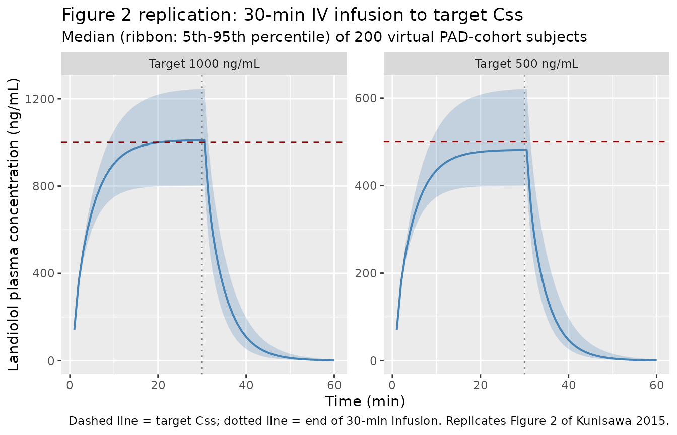
The model reaches the target plasma concentration within roughly five elimination half-lives (about 15-20 min) and washes out almost completely within 20 min of infusion end, consistent with landiolol’s ultra-short-acting profile (terminal half-life ~3-4 min reported in the source).
PKNCA validation
A single 30-min infusion is sufficient to characterise distribution
(tmax, cmax), exposure (auclast,
aucinf.obs), and terminal elimination
(half.life). The PKNCA formula stratifies by
target_ngml so per-group steady-state and washout
properties are visible.
sim_nca <- sim |>
  dplyr::filter(!is.na(Cc)) |>
  dplyr::select(id, time, Cc, target_ngml) |>
  dplyr::mutate(target_ngml = as.character(target_ngml))

conc_obj <- PKNCA::PKNCAconc(sim_nca, Cc ~ time | target_ngml + id)

dose_df <- events |>
  dplyr::filter(evid == 1) |>
  dplyr::select(id, time, amt, rate, target_ngml) |>
  dplyr::mutate(
    duration    = amt / rate,                    # infusion duration in hours
    target_ngml = as.character(target_ngml)
  )

dose_obj <- PKNCA::PKNCAdose(
  dose_df,
  amt ~ time | target_ngml + id,
  duration = "duration"
)

intervals <- data.frame(
  start      = 0,
  end        = 1,                                # 60 min in hours
  cmax       = TRUE,
  tmax       = TRUE,
  auclast    = TRUE,
  aucinf.obs = TRUE,
  half.life  = TRUE
)

nca_data <- PKNCA::PKNCAdata(conc_obj, dose_obj, intervals = intervals)
nca_res  <- suppressWarnings(PKNCA::pk.nca(nca_data))
nca_summary <- summary(nca_res)
knitr::kable(nca_summary,
caption = "Simulated NCA parameters by TCI target (median and inter-quartile range across 200 virtual subjects).")| start | end | target_ngml | N | auclast | cmax | tmax | half.life | aucinf.obs |
|---|---|---|---|---|---|---|---|---|
| 0 | 1 | 1000 | 200 | NC | 1010 [14.4] | 0.508 [0.508, 0.508] | 0.0526 [0.00645] | NC |
| 0 | 1 | 500 | 200 | NC | 494 [13.9] | 0.508 [0.508, 0.508] | 0.0516 [0.00623] | NC |
Comparison against published values
Kunisawa 2015 does not report subject-level NCA, but does state the landiolol terminal half-life is approximately 4 minutes (Introduction) and describes a 64-84% reduction in Vc and CL relative to healthy volunteers (Conclusion). The simulated steady-state plasma concentration during the 30-min infusion clusters around each TCI target value (500 or 1,000 ng/mL).
# Expected terminal half-life derived from the typical-value 2-cmt parameters
# at 70 kg reference: alpha + beta = k10 + k12 + k21; alpha * beta = k10 * k21.
cl70 <- 128.94; vc70 <- 4.55; q70 <- 202.86; vp70 <- 3.808
kel  <- cl70 / vc70
k12  <- q70  / vc70
k21  <- q70  / vp70
ab_sum  <- kel + k12 + k21
ab_prod <- kel * k21
discr   <- sqrt(ab_sum^2 - 4 * ab_prod)
alpha   <- (ab_sum + discr) / 2
beta    <- (ab_sum - discr) / 2
t_half_alpha_min <- log(2) / alpha * 60
t_half_beta_min  <- log(2) / beta  * 60

tibble(
  metric = c("Distribution half-life t1/2,alpha (min)",
             "Terminal half-life t1/2,beta (min)",
             "Steady-state Css at 500-ng/mL target (ng/mL)",
             "Steady-state Css at 1000-ng/mL target (ng/mL)"),
  expected = c(round(t_half_alpha_min, 2), round(t_half_beta_min, 2), 500, 1000),
  paper = c("not reported (typical 2-cmt distribution)",
            "~4 (Introduction)",
            "500 (Methods/Figure 1)",
            "1000 (Methods/Figure 1)")
) |>
knitr::kable(caption = "Expected vs. paper-reported PK metrics.")| metric | expected | paper |
|---|---|---|
| Distribution half-life t1/2,alpha (min) | 0.37 | not reported (typical 2-cmt distribution) |
| Terminal half-life t1/2,beta (min) | 3.11 | ~4 (Introduction) |
| Steady-state Css at 500-ng/mL target (ng/mL) | 500.00 | 500 (Methods/Figure 1) |
| Steady-state Css at 1000-ng/mL target (ng/mL) | 1000.00 | 1000 (Methods/Figure 1) |
Assumptions and deviations
-
TCI replicated as constant infusion. The published
study used a closed-loop Target-Controlled Infusion (TCI) algorithm
under STANPUMP, computing a time-varying infusion rate per Honda et al’s
parameters to drive plasma to 500 and 1,000 ng/mL targets. The vignette
approximates this with a single constant infusion at the rate
target_ngml * 30.7 mL/min/kg(i.e., the steady-state rate fromCss = rate / CL) using the typical-value clearance. The actual TCI trajectory would include a brief loading bolus and online rate adjustment; the steady-state plateau is the same. - Body-weight distribution. Cohort weights drawn from a log-normal distribution matched to the published mean and SD, clipped to the observed range 40.4-71.8 kg (Table 1) to avoid extrapolation. The source paper reports body weight, lean body mass, and age as candidate covariates but none were retained beyond the linear per-kg normalization baked into the structural model.
- Race / ethnicity. All cohort subjects were Japanese (Asahikawa Medical University). The model does not include race as a covariate; predictions in non-Japanese populations should be made cautiously until a confirmatory study is available.
- Co-medication / surgical context. Parameters were estimated under general anaesthesia with concomitant TCI propofol, TCI remifentanil, rocuronium, and continuous dopamine 3 ug/kg/min. The paper warns (Discussion) that PK in PAD patients may differ in other clinical settings.
- Mildly abnormal laboratory values. Some subjects had mildly abnormal albumin, cholinesterase, BUN, or serum creatinine; these were not retained as covariates because of the limited frequency and extent of abnormalities (Results).
-
Residual error mapping. The paper describes the
residual error as an “exponential error model”; nlmixr2’s
lnorm()is the direct equivalent of NONMEMY = F * EXP(EPS).expSd = sqrt(0.0773) = 0.278on the log scale. - Pages 107-114, Therapeutics and Clinical Risk Management 2015;11. Open access (Dove Press, CC BY-NC 3.0); DOI 10.2147/TCRM.S74867.