GCC-4401C and rivaroxaban PK/PD (Choi 2016)
Source:vignettes/articles/Choi_2016_gcc4401c_rivaroxaban.Rmd
Choi_2016_gcc4401c_rivaroxaban.RmdModels and source
Choi 2016 pooled two phase I trials of the oral direct factor Xa inhibitor GCC-4401C and fit, side by side, a population PK/PD model for GCC-4401C and one for the rivaroxaban active-comparator arm. The two fits share no parameters and were built on different cohorts, so the paper contributes two model files:
mod_gcc <- readModelDb("Choi_2016_gcc4401c")
mod_riv <- readModelDb("Choi_2016_rivaroxaban")
ui_gcc <- rxode2::rxode(mod_gcc)
#> ℹ parameter labels from comments will be replaced by 'label()'
#> Warning: some etas defaulted to non-mu referenced, possible parsing error: etaiov_d1_1, etaiov_d1_2, etaiov_d1_3, etaiov_d1_4, etaiov_d1_5, etaiov_d1_6, etaiov_d1_7, etaiov_tlag_1, etaiov_tlag_2, etaiov_tlag_3, etaiov_tlag_4, etaiov_tlag_5, etaiov_tlag_6, etaiov_tlag_7, etaiov_hill_cfx_1, etaiov_hill_cfx_2, etaiov_hill_cfx_3, etaiov_hill_ptinr_1, etaiov_hill_ptinr_2, etaiov_hill_ptinr_3, etaiov_hill_ptsec_1, etaiov_hill_ptsec_2, etaiov_hill_ptsec_3, etaiov_hill_aptt_1, etaiov_hill_aptt_2, etaiov_hill_aptt_3
#> as a work-around try putting the mu-referenced expression on a simple line
ui_riv <- rxode2::rxode(mod_riv)
#> ℹ parameter labels from comments will be replaced by 'label()'
#> Warning: some etas defaulted to non-mu referenced, possible parsing error: etaiov_d1_1, etaiov_d1_2, etaiov_d1_3, etaiov_d1_4, etaiov_d1_5, etaiov_d1_6, etaiov_d1_7, etaiov_ec50_cfx_1, etaiov_ec50_cfx_2, etaiov_ec50_cfx_3, etaiov_ec50_fxcaa_1, etaiov_ec50_fxcaa_2, etaiov_ec50_fxcaa_3
#> as a work-around try putting the mu-referenced expression on a simple line- Citation: Choi HY, Choi S, Kim YH, Lim HS. Population pharmacokinetic and pharmacodynamic modeling analysis of GCC-4401C, a novel direct factor Xa inhibitor, in healthy volunteers. CPT Pharmacometrics Syst Pharmacol. 2016 Oct;5(10):532-543. doi:10.1002/psp4.12103. Structural detail and the plasma/urine NONMEM control stream are taken from Supplementary Data file PSP4-5-532-s008 accompanying the article; the coagulation-factor-X PD control stream is PSP4-5-532-s009.
- GCC-4401C: Population PK/PD model for GCC-4401C, an oral direct factor Xa inhibitor, in healthy male volunteers (Choi 2016; pooled first-in-human single-ascending-dose and single-and-multiple-ascending-dose phase I studies). Plasma and urine data were fit simultaneously with a two-compartment model with sequential zero-order release into the depot (D1), an absorption lag (ALAG1) and first-order absorption; body weight enters Vc as a power function normalised to 75 kg. Elimination is split into a linear non-renal clearance and a saturable renal clearance whose magnitude is suppressed by an inhibitory Emax function of the plasma concentration. A study-specific scaling of the apparent Vc encodes the relative accuracy of the two bioanalytical assays. Eight pharmacodynamic markers are carried as direct-effect (no-delay) outputs driven by the plasma concentration: coagulation factor X activity, factor X chromogenic activity, anti-factor Xa activity, prothrombin time in INR and in seconds, activated partial thromboplastin time, antithrombin III activity and the low-molecular-weight-heparin anti-Xa assay. The PD layer was fit sequentially on individual Bayesian PK estimates. Baselines for aPTT, AT III and LMWH are not reported anywhere in the paper or its supplement, so those three outputs are the drug-induced CHANGE from baseline and are named with a _chg suffix; see the vignette Errata. Companion rivaroxaban model: modellib(‘Choi_2016_rivaroxaban’).
- Rivaroxaban: Population PK/PD model for rivaroxaban 20 mg once daily taken with food in healthy male volunteers, fit as the active comparator arm of the GCC-4401C single-and-multiple-ascending-dose phase I study (Choi 2016). Disposition is two-compartment with linear clearance; absorption is a Weibull-type process (shape gamma) combined with zero-order release into the depot over a duration D1, with no absorption lag and no retained covariates. Six pharmacodynamic markers are carried as direct-effect (no-delay) outputs driven by the plasma concentration: coagulation factor X activity, factor X chromogenic activity, anti-factor Xa activity, prothrombin time in INR and in seconds, and activated partial thromboplastin time. The PD layer was fit sequentially on individual Bayesian PK estimates. The baseline aPTT is not reported anywhere in the paper or its supplement, so that output is the drug-induced CHANGE from baseline and is named with a _chg suffix; see the vignette Errata. Companion GCC-4401C model: modellib(‘Choi_2016_gcc4401c’).
- Article: https://doi.org/10.1002/psp4.12103
- Supplementary data (open access, includes the plasma/urine and coagulation-factor-X NONMEM control streams and the simulation figures used below): https://europepmc.org/article/PMC/PMC5080649
Population
Ninety-four healthy male volunteers took part in the two trials: 48 in the first-in-human single-ascending-dose study (SAD, NCT01651234; six dose groups of eight, 2.5 to 80 mg, six active and two placebo per group) and 46 in the single- and-multiple-ascending-dose study (S&MAD, NCT01954238; five dose groups of eight, 10 to 80 mg, dosed on day 1 and on days 3 through 9). Mean (SD) age was 30.3 (8.6) years, weight 76.6 (9.7) kg and height 176.5 (6.7) cm; 43.6% were White, 42.6% African American, 8.5% Asian and 5.3% other (Choi 2016 Table 1). An extra six subjects in the 20 mg S&MAD group received rivaroxaban 20 mg 30 minutes after a standard breakfast and form the entire rivaroxaban cohort.
GCC-4401C was given fasted and rivaroxaban fed, as its label recommends. That difference is deliberate and is the reason the paper’s dose-equivalence conclusions are framed as “20 mg and 40 mg of GCC-4401C administered under fasted status are comparable to 10 mg and 20 mg of rivaroxaban under fed status”.
The PK dataset held 1,401 plasma GCC-4401C concentrations, 120 urine concentrations and 168 plasma rivaroxaban concentrations. The same metadata is available programmatically:
str(ui_gcc$population, max.level = 1)
#> List of 13
#>  $ species       : chr "human"
#>  $ n_subjects    : int 94
#>  $ n_studies     : int 2
#>  $ n_observations: int 1689
#>  $ age_range     : chr "mean (SD) 30.3 (8.6) years"
#>  $ weight_range  : chr "mean (SD) 76.6 (9.7) kg"
#>  $ height_range  : chr "mean (SD) 176.5 (6.7) cm"
#>  $ sex_female_pct: num 0
#>  $ race_ethnicity: Named num [1:4] 43.6 42.6 8.5 5.3
#>   ..- attr(*, "names")= chr [1:4] "White" "Black" "Asian" "Other"
#>  $ disease_state : chr "Healthy male volunteers."
#>  $ dose_range    : chr "Single oral doses of 2.5, 5, 10, 20, 40 or 80 mg under overnight fasting (SAD study, 48 subjects, 6 active + 2 "| __truncated__
#>  $ regions       : chr "United States (ClinicalTrials.gov NCT01651234 and NCT01954238)."
#>  $ notes         : chr "Baseline demographics from Choi 2016 Table 1; the two studies did not differ materially. PK dataset: 1401 plasm"| __truncated__
Source trace
Every ini() entry carries an in-file comment naming its
source location. The table below collects the structural entries; the
per-parameter table locations are in
inst/modeldb/specificDrugs/Choi_2016_gcc4401c.R and
inst/modeldb/specificDrugs/Choi_2016_rivaroxaban.R.
| Element | Source location |
|---|---|
| GCC-4401C two-compartment disposition, zero-order depot release (D1) + lag (ALAG1) + first-order absorption | Results “Plasma and urine PK modeling analysis”; supplementary
control stream PSP4-5-532-s008 $MODEL /
$PK / $DES
|
Typical Vc = Vc(75) * (WT/75)^H |
Equation 5; Table 2(a) |
CLR = BCLR * (1 - IMAX * Cp / (Cp + IC50)) (saturable
renal clearance) |
Equation 6; control stream $DES
K24 = CLR*(1 - IMX*C2/(C2 + IC50))/V2
|
S2 = Vc/1000, and S2 = (Vc/1000)/THETA(10)
for the S&MAD study |
Equations 7 and 8; Table 2(a) footnote d |
| All GCC-4401C PK point estimates and IIV variances | Table 2(a) |
| Rivaroxaban two-compartment disposition, Weibull absorption + zero-order D1 | Results “For rivaroxaban, a two-compartment, linear model best described the PK in fed status”; Table 2(b) |
| All rivaroxaban PK point estimates and IIV variances | Table 2(b) |
Direct-effect PD form
E = BASE -/+ Emax * Cc^gamma / (EC50^gamma + Cc^gamma)
|
PD control stream PSP4-5-532-s009 $ERROR
CFX = BASE - EMAX*(CP**GAM)/(EC50**GAM+CP**GAM)
|
| Absence of a PD time delay | Results “PK-PD modeling analysis”: no counterclockwise hysteresis; association-dissociation models not superior to direct-effect models |
| All PD point estimates, IIV and IOV variances, residual errors | Table 3(a)-(h) |
| Typical baselines for CFX, FXCAA, AFX, PT (INR) and PT (s) | Digitised from Supplementary Figure S4 (pre-dose median of each panel) – see Errata |
| Occasion structure for IOV | Results “IOVs for D1 and ALAG1 … implemented in every inter-dose
interval”; seven $OMEGA BLOCK(1) SAME slots in
PSP4-5-532-s008, three in PSP4-5-532-s009
|
Simulation helpers
Both models are multi-endpoint, so observation records carry the
endpoint name in cmt. useLinCmt = FALSE keeps
rxode2 from attempting an ODE-to-linCmt() conversion that
would discard the custom absorption structure.
# Typical-value (population) profiles: omega = NA suppresses all random effects.
solve_typical <- function(ui, dose, times, extra = list(), addl = NULL, ii = NULL) {
  ev <- rxode2::et(amt = dose, rate = -2, cmt = "depot")
  if (!is.null(addl)) ev <- rxode2::et(amt = dose, rate = -2, cmt = "depot", addl = addl, ii = ii)
  ev <- ev |> rxode2::et(times, cmt = "Cc")
  ev <- as.data.frame(ev)
  for (nm in names(extra)) ev[[nm]] <- extra[[nm]]
  rxode2::rxSolve(ui, ev, omega = NA, useLinCmt = FALSE, returnType = "data.frame")
}

trapz <- function(t, y) sum(diff(t) * (utils::head(y, -1) + utils::tail(y, -1)) / 2)

grid_sd <- seq(0, 168, by = 0.05)
Single-dose typical profiles
gcc_doses <- c(2.5, 5, 10, 20, 40, 80)

sd_gcc <- lapply(gcc_doses, function(d) {
  solve_typical(ui_gcc, d, grid_sd,
    extra = list(WT = 75, STUDY_SMAD = 0, OCC = 1)
  ) |>
    dplyr::mutate(drug = "GCC-4401C", study = "SAD", dose = d)
}) |> dplyr::bind_rows()

sd_gcc_smad <- lapply(c(10, 20, 40), function(d) {
  solve_typical(ui_gcc, d, grid_sd,
    extra = list(WT = 75, STUDY_SMAD = 1, OCC = 1)
  ) |>
    dplyr::mutate(drug = "GCC-4401C", study = "S&MAD", dose = d)
}) |> dplyr::bind_rows()

sd_riv <- lapply(c(10, 20), function(d) {
  solve_typical(ui_riv, d, grid_sd, extra = list(OCC = 1)) |>
    dplyr::mutate(drug = "Rivaroxaban", study = "S&MAD", dose = d)
}) |> dplyr::bind_rows()

# rxode2 must never return a negative concentration here: there is no
# stiff transient and PKNCA would silently produce NaN AUCs if it did.
stopifnot(
  min(sd_gcc$Cc) >= 0, min(sd_gcc_smad$Cc) >= 0, min(sd_riv$Cc) >= 0,
  !anyNA(sd_gcc$Cc), !anyNA(sd_riv$Cc)
)
Replicate published figures
Figure 2a – GCC-4401C plasma, single ascending dose
Figure 2a is a prediction-corrected VPC standardised to a 40 mg dose,
so the comparable quantity is the median of a simulated
cohort, not the typical-value curve. The paper’s IIV on
Ka is very large (variance 0.97, CV 128%), which pulls the
cohort median below the typical-value profile.
# `set.seed()` seeds R's RNG, not rxode2's; rxode2 partitions its streams per
# solver thread, so this cohort differs between a 16-thread workstation and a
# 2-core CI runner. Every assertion below is written to hold for any cohort.
set.seed(20161011)
n_sub <- 100L

cohort <- tibble::tibble(
  id = seq_len(n_sub),
  WT = pmin(pmax(stats::rnorm(n_sub, 76.6, 9.7), 50), 120), # Table 1: 76.6 (9.7) kg
  STUDY_SMAD = 0,
  OCC = 1
)

obs_times <- seq(0, 48, by = 0.25)

ev_vpc <- dplyr::bind_rows(
  cohort |> dplyr::mutate(
    time = 0, evid = 1L, amt = 40, rate = -2, cmt = "depot"
  ),
  tidyr::expand_grid(cohort, time = obs_times) |>
    dplyr::mutate(evid = 0L, amt = NA_real_, rate = NA_real_, cmt = "Cc")
) |>
  dplyr::arrange(id, time, dplyr::desc(evid))
stopifnot(!anyDuplicated(unique(ev_vpc[, c("id", "time", "evid")])))

vpc <- rxode2::rxSolve(ui_gcc, ev_vpc, keep = c("WT"), useLinCmt = FALSE) |>
  as.data.frame()

vpc_q <- vpc |>
  dplyr::group_by(time) |>
  dplyr::summarise(
    Q025 = stats::quantile(Cc, 0.025, na.rm = TRUE),
    Q50 = stats::quantile(Cc, 0.50, na.rm = TRUE),
    Q975 = stats::quantile(Cc, 0.975, na.rm = TRUE),
    .groups = "drop"
  )

typ40 <- sd_gcc |> dplyr::filter(dose == 40, time <= 48)

ggplot(vpc_q, aes(time, Q50)) +
  geom_ribbon(aes(ymin = Q025, ymax = Q975), alpha = 0.25, fill = "steelblue") +
  geom_line(linewidth = 0.9, colour = "steelblue") +
  geom_line(data = typ40, aes(time, Cc), colour = "firebrick", linetype = 2) +
  labs(
    x = "Time (h)", y = "GCC-4401C plasma concentration (ng/mL)",
    title = "Figure 2a - GCC-4401C 40 mg, single dose",
    subtitle = "Blue: simulated cohort median and 95% interval. Red dashed: typical-value profile.",
    caption = "Replicates Figure 2a (left panel) of Choi 2016."
  )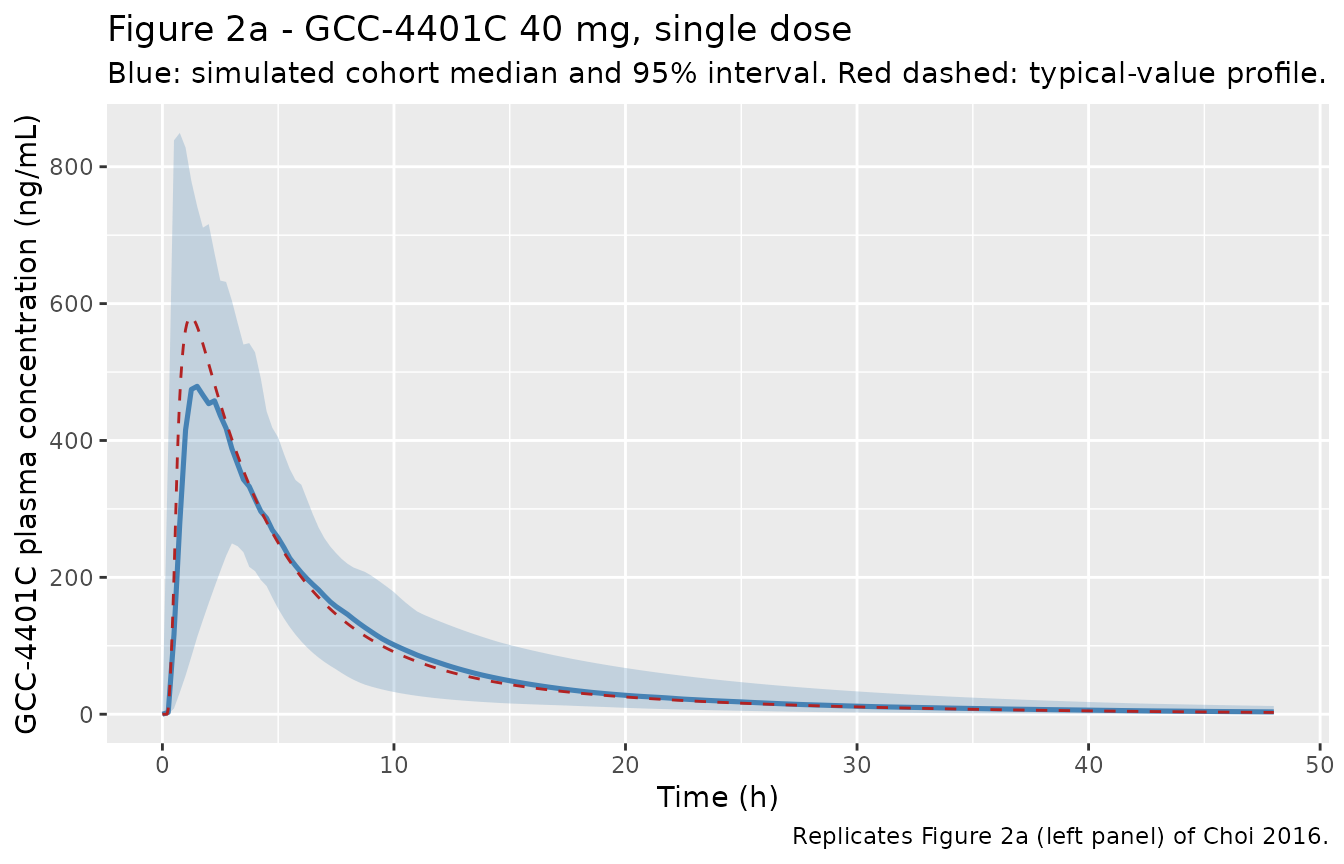
Figure 2b – GCC-4401C cumulative urinary excretion
The saturable renal clearance is the most distinctive feature of this model, and the cumulative urine curve is the only place it is directly observable. Figure 2b is standardised to 40 mg and plateaus at roughly 1,400 ug.
ae_plot <- sd_gcc |>
  dplyr::filter(dose %in% c(10, 20, 40, 80), time <= 48) |>
  dplyr::mutate(Ae_ug = 1000 * Ae, dose_lab = factor(paste(dose, "mg"),
    levels = paste(c(10, 20, 40, 80), "mg")
  ))

ggplot(ae_plot, aes(time, Ae_ug, colour = dose_lab)) +
  geom_line(linewidth = 0.8) +
  labs(
    x = "Time after dose (h)", y = "Cumulative GCC-4401C in urine (ug)",
    colour = "Dose",
    title = "Figure 2b - cumulative urinary excretion of GCC-4401C",
    caption = "Replicates Figure 2b of Choi 2016 (which is standardised to 40 mg)."
  )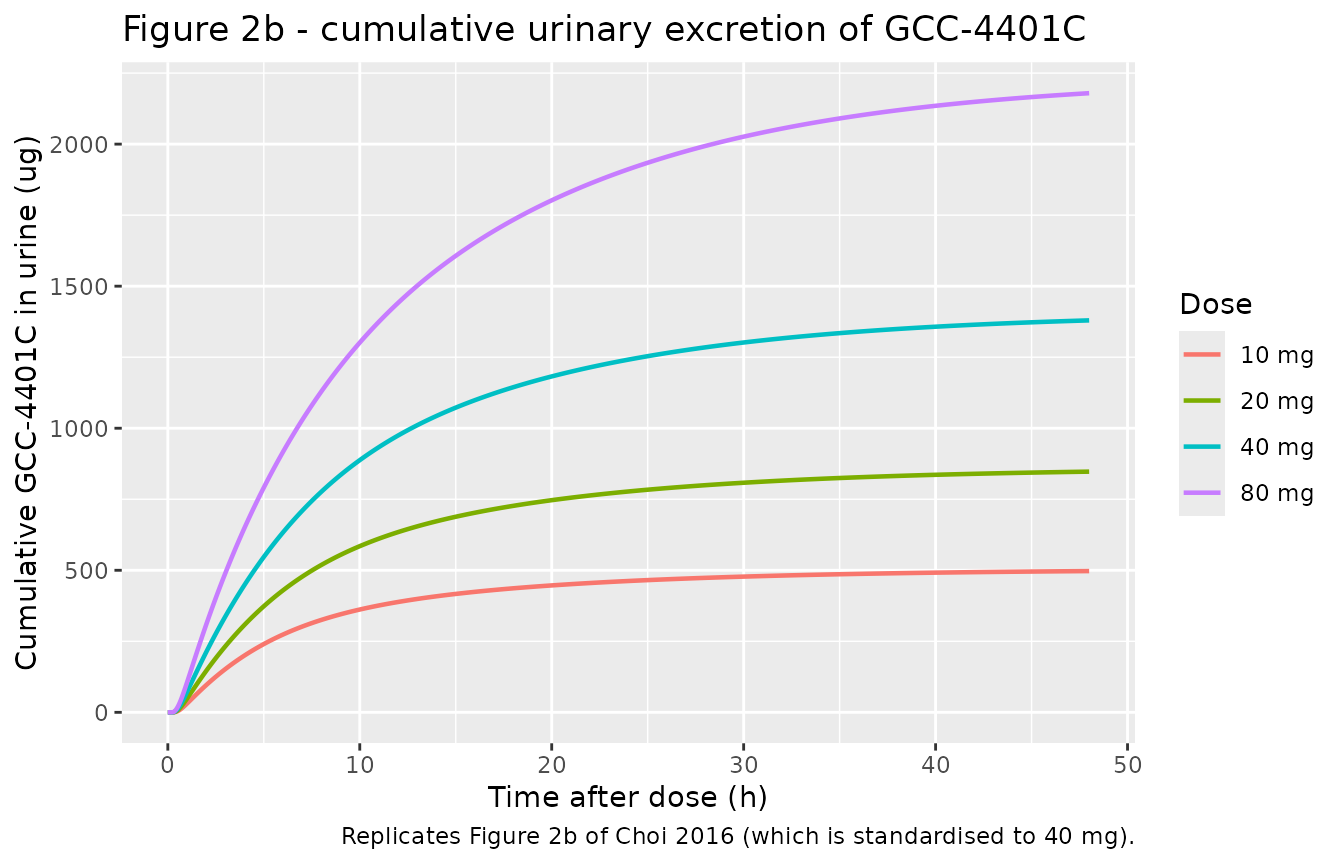
Figure 2c – rivaroxaban plasma, 20 mg
sd_riv |>
  dplyr::filter(dose == 20, time <= 48) |>
  ggplot(aes(time, Cc)) +
  geom_line(linewidth = 0.9, colour = "darkorange") +
  labs(
    x = "Time (h)", y = "Rivaroxaban plasma concentration (ng/mL)",
    title = "Figure 2c - rivaroxaban 20 mg, typical-value profile",
    caption = "Replicates Figure 2c of Choi 2016."
  )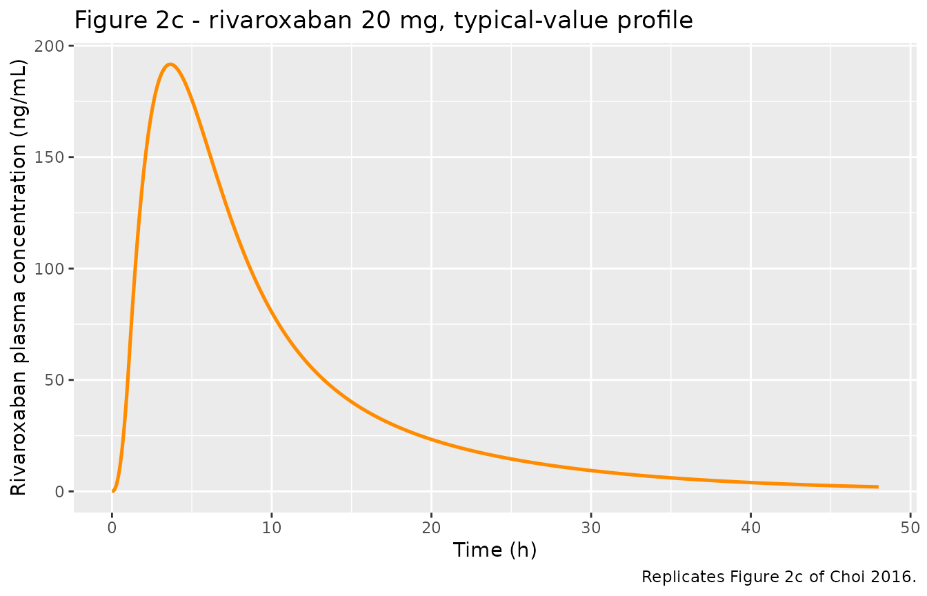
Figure 4 and Supplementary Figure S4 – PD markers over a once-daily week
Figure 4 and Supplementary Figure S4 simulate once-daily dosing for seven days and overlay GCC-4401C against rivaroxaban. The occasion index advances one per dosing day, which is how the model’s inter-occasion variability is indexed.
grid_md <- seq(0, 168, by = 0.1)
occ_md <- pmin(floor(grid_md / 24) + 1, 7)

solve_md <- function(ui, dose, extra) {
  ev <- rxode2::et(amt = dose, rate = -2, cmt = "depot", addl = 6, ii = 24) |>
    rxode2::et(grid_md, cmt = "Cc")
  ev <- as.data.frame(ev)
  ev$OCC <- pmin(floor(ev$time / 24) + 1, 7)
  for (nm in names(extra)) ev[[nm]] <- extra[[nm]]
  rxode2::rxSolve(ui, ev, omega = NA, useLinCmt = FALSE, returnType = "data.frame")
}

md <- dplyr::bind_rows(
  solve_md(ui_gcc, 20, list(WT = 75, STUDY_SMAD = 1)) |>
    dplyr::mutate(arm = "GCC-4401C 20 mg", pair = "GCC 20 mg vs rivaroxaban 10 mg"),
  solve_md(ui_riv, 10, list()) |>
    dplyr::mutate(arm = "Rivaroxaban 10 mg", pair = "GCC 20 mg vs rivaroxaban 10 mg"),
  solve_md(ui_gcc, 40, list(WT = 75, STUDY_SMAD = 1)) |>
    dplyr::mutate(arm = "GCC-4401C 40 mg", pair = "GCC 40 mg vs rivaroxaban 20 mg"),
  solve_md(ui_riv, 20, list()) |>
    dplyr::mutate(arm = "Rivaroxaban 20 mg", pair = "GCC 40 mg vs rivaroxaban 20 mg")
)

md_long <- md |>
  dplyr::select(time, arm, pair, cfx, fxcaa, afx, ptinr) |>
  tidyr::pivot_longer(c(cfx, fxcaa, afx, ptinr), names_to = "marker", values_to = "value") |>
  dplyr::mutate(marker = factor(marker,
    levels = c("cfx", "fxcaa", "afx", "ptinr"),
    labels = c(
      "Coagulation factor X (%)", "Factor X chromogenic (%)",
      "Anti-factor Xa (IU/mL)", "Prothrombin time (INR)"
    )
  ))

ggplot(md_long, aes(time, value, colour = arm)) +
  geom_line(linewidth = 0.7) +
  facet_grid(marker ~ pair, scales = "free_y") +
  scale_x_continuous(breaks = seq(0, 168, by = 48)) +
  labs(
    x = "Time (h)", y = NULL, colour = NULL,
    title = "Figure 4 / Supplementary Figure S4 - PD markers, once daily for 7 days",
    caption = "Replicates Figure 4 and Supplementary Figure S4 of Choi 2016 (typical-value curves)."
  ) +
  theme(legend.position = "bottom")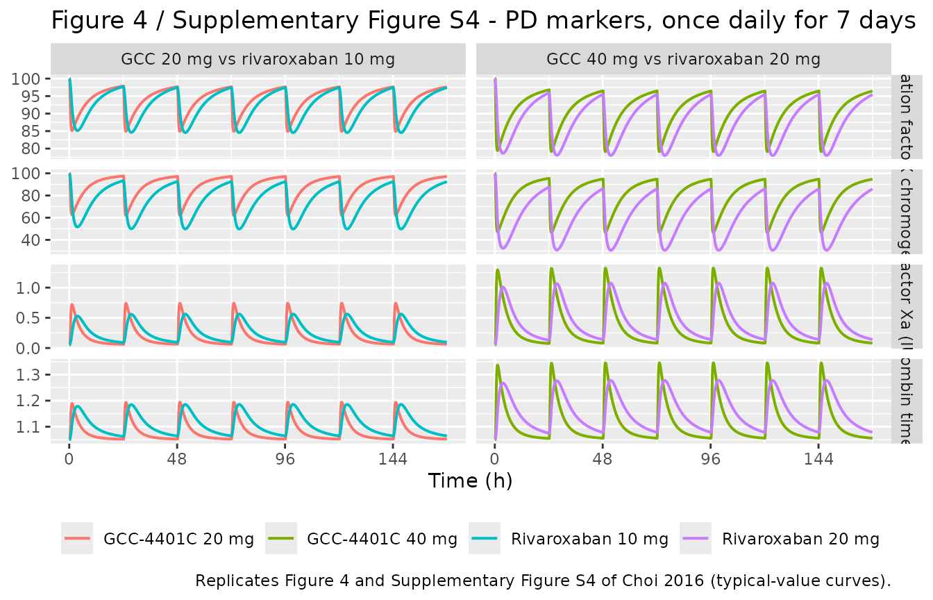
PKNCA validation
The paper reports no non-compartmental analysis table, so PKNCA is used here to derive exposure metrics that can be checked against the two quantities the paper does print: the total clearances (12.0 L/h for GCC-4401C, 10.1 L/h for rivaroxaban, Results “Monte-Carlo simulation”) and the split of GCC-4401C clearance into non-renal (11.2 L/h) and renal (0.78 L/h) arms (Table 2a).
nca_input <- dplyr::bind_rows(sd_gcc, sd_riv) |>
  dplyr::mutate(arm = paste0(drug, " ", dose, " mg")) |>
  dplyr::filter(!is.na(Cc)) |>
  dplyr::mutate(id = arm) |>
  dplyr::select(id, time, Cc, arm)

# Guarantee a time = 0 record per arm so AUC0-* is anchored (both drugs are
# extravascular, so the pre-dose concentration is exactly 0).
nca_input <- dplyr::bind_rows(
  nca_input,
  nca_input |> dplyr::distinct(id, arm) |> dplyr::mutate(time = 0, Cc = 0)
) |>
  dplyr::distinct(id, arm, time, .keep_all = TRUE) |>
  dplyr::arrange(id, time)
stopifnot(nrow(nca_input) > 0, all(table(nca_input$arm) > 100))

dose_df <- dplyr::bind_rows(sd_gcc, sd_riv) |>
  dplyr::mutate(arm = paste0(drug, " ", dose, " mg")) |>
  dplyr::distinct(id = arm, arm, amt = dose) |>
  dplyr::mutate(time = 0)

conc_obj <- PKNCA::PKNCAconc(nca_input, Cc ~ time | arm + id)
dose_obj <- PKNCA::PKNCAdose(dose_df, amt ~ time | arm + id)

intervals <- data.frame(
  start = 0, end = Inf,
  cmax = TRUE, tmax = TRUE, auclast = TRUE, aucinf.obs = TRUE, half.life = TRUE
)

nca_res <- PKNCA::pk.nca(PKNCA::PKNCAdata(conc_obj, dose_obj, intervals = intervals))

nca_tab <- as.data.frame(nca_res) |>
  dplyr::select(arm, PPTESTCD, PPORRES) |>
  tidyr::pivot_wider(names_from = PPTESTCD, values_from = PPORRES)

nca_tab |>
  dplyr::transmute(
    arm,
    cmax = round(cmax, 1), tmax = round(tmax, 2),
    auclast = round(auclast, 0), aucinf.obs = round(aucinf.obs, 0),
    half.life = round(half.life, 2)
  ) |>
  dplyr::rename(
    "Arm" = arm,
    "Cmax (ng/mL)" = cmax,
    "Tmax (h)" = tmax,
    "AUC0-168 (ng*h/mL)" = auclast,
    "AUC0-inf (ng*h/mL)" = aucinf.obs,
    "t1/2 (h)" = half.life
  ) |>
knitr::kable(caption = "PKNCA metrics from the typical-value single-dose profiles.")| Arm | Cmax (ng/mL) | Tmax (h) | AUC0-168 (ng*h/mL) | AUC0-inf (ng*h/mL) | t1/2 (h) |
|---|---|---|---|---|---|
| GCC-4401C 10 mg | 144.7 | 1.25 | 848 | 848 | 8.92 |
| GCC-4401C 2.5 mg | 36.1 | 1.20 | 210 | 210 | 8.92 |
| GCC-4401C 20 mg | 289.8 | 1.25 | 1709 | 1709 | 8.92 |
| GCC-4401C 40 mg | 580.2 | 1.25 | 3446 | 3446 | 8.91 |
| GCC-4401C 5 mg | 72.3 | 1.20 | 421 | 421 | 8.92 |
| GCC-4401C 80 mg | 1161.3 | 1.25 | 6943 | 6944 | 8.91 |
| Rivaroxaban 10 mg | 95.8 | 3.65 | 990 | 990 | 8.10 |
| Rivaroxaban 20 mg | 191.6 | 3.65 | 1980 | 1980 | 8.10 |
Closed-form exposure gate
For rivaroxaban the model is linear, so AUC0-inf must
equal Dose / CL exactly. For GCC-4401C the renal arm
saturates, so the observed clearance must sit between
the non-renal-only clearance (11.2 L/h, the limit at concentrations far
above IC50) and the total clearance (11.98 L/h, the limit at
concentrations far below it) – and must approach the lower clearance as
the dose rises. That monotone drift is the signature of Equation 6 and
is what this gate protects.
cl_obs <- nca_tab |>
  dplyr::left_join(dose_df |> dplyr::select(arm, amt), by = "arm") |>
  dplyr::mutate(
    cl_apparent = 1000 * amt / aucinf.obs,
    drug = ifelse(grepl("^GCC", arm), "GCC-4401C", "Rivaroxaban")
  )

cl_obs |>
  dplyr::transmute(arm,
    `Dose (mg)` = amt,
    `Apparent CL from AUC0-inf (L/h)` = round(cl_apparent, 3)
  ) |>
knitr::kable(caption = "Apparent clearance recovered from the simulated AUC0-inf.")| arm | Dose (mg) | Apparent CL from AUC0-inf (L/h) |
|---|---|---|
| GCC-4401C 10 mg | 10.0 | 11.794 |
| GCC-4401C 2.5 mg | 2.5 | 11.916 |
| GCC-4401C 20 mg | 20.0 | 11.703 |
| GCC-4401C 40 mg | 40.0 | 11.608 |
| GCC-4401C 5 mg | 5.0 | 11.867 |
| GCC-4401C 80 mg | 80.0 | 11.522 |
| Rivaroxaban 10 mg | 10.0 | 10.100 |
| Rivaroxaban 20 mg | 20.0 | 10.100 |
riv_cl <- cl_obs$cl_apparent[cl_obs$drug == "Rivaroxaban"]
gcc_cl <- cl_obs |>
  dplyr::filter(drug == "GCC-4401C") |>
  dplyr::arrange(amt)

stopifnot(
  # Rivaroxaban: linear, so the recovered CL must be the published 10.1 L/h.
  # Deterministic (omega = NA), so a tight bound is correct here.
  all(abs(riv_cl - 10.1) / 10.1 < 0.01),
  # GCC-4401C: bracketed by CLNR alone and by CLNR + CLR, and monotonically
  # falling toward CLNR as the dose (and so the renal saturation) rises.
  all(gcc_cl$cl_apparent > 11.2), all(gcc_cl$cl_apparent < 11.98 * 1.001),
  all(diff(gcc_cl$cl_apparent) < 0)
)
Renal mass balance
fe <- sd_gcc |>
  dplyr::group_by(dose) |>
  dplyr::summarise(fe_pct = 100 * max(Ae) / dplyr::first(dose), .groups = "drop") |>
  dplyr::arrange(dose)

fe |>
  dplyr::transmute(`Dose (mg)` = dose, `Fraction excreted unchanged in urine (%)` = round(fe_pct, 2)) |>
knitr::kable(caption = "Cumulative urinary recovery over 168 h.")| Dose (mg) | Fraction excreted unchanged in urine (%) |
|---|---|
| 2.5 | 6.01 |
| 5.0 | 5.62 |
| 10.0 | 5.04 |
| 20.0 | 4.30 |
| 40.0 | 3.51 |
| 80.0 | 2.79 |
Study assay-scaling gate
The S&MAD study’s concentrations are scaled by a factor of 0.82
relative to the SAD study (Table 2a “Assay”; Equations 7-8). The scaling
divides the apparent volume, so – exactly as in the supplementary
control stream, where S2 is what $DES uses to
form C2 – the scaled concentration is also the one that
drives the saturable renal clearance. The ratio is therefore
not a flat 0.82: it starts at 0.82 and drifts slightly
below it, because the S&MAD study’s lower apparent concentration
saturates the renal route less and so eliminates a little faster.
That drift is a feature worth gating rather than an error to
tolerate. It must be small (the renal arm is only
0.78 / 11.98 = 6.5% of total clearance), it must be
one-sided (feedback can only reduce the ratio), and it must
grow with dose, since higher concentrations mean more
renal saturation in the SAD arm to undo. All three are asserted below.
The solve is deterministic (omega = NA), so tight bounds
are correct here.
ratio <- sd_gcc_smad |>
  dplyr::filter(dose %in% c(10, 20, 40)) |>
  dplyr::select(time, dose, Cc_smad = Cc) |>
  dplyr::inner_join(
    sd_gcc |> dplyr::filter(dose %in% c(10, 20, 40)) |> dplyr::select(time, dose, Cc_sad = Cc),
    by = c("time", "dose")
  ) |>
  dplyr::filter(Cc_sad > 1) |>
  dplyr::mutate(ratio = Cc_smad / Cc_sad)

ratio_by_dose <- ratio |>
  dplyr::group_by(dose) |>
  dplyr::summarise(
    n = dplyr::n(),
    min_ratio = min(ratio),
    max_ratio = max(ratio),
    max_drift = max(0.82 - ratio),
    .groups = "drop"
  ) |>
  dplyr::arrange(dose)

ratio_by_dose |>
  dplyr::transmute(
    `Dose (mg)` = dose,
    `Ratio, min` = round(min_ratio, 6),
    `Ratio, max` = round(max_ratio, 6),
    `Max drift below 0.82` = signif(max_drift, 3)
  ) |>
knitr::kable(caption = "S&MAD / SAD concentration ratio (nominal assay factor 0.82).")| Dose (mg) | Ratio, min | Ratio, max | Max drift below 0.82 |
|---|---|---|---|
| 10 | 0.817038 | 0.820000 | 0.00296 |
| 20 | 0.816171 | 0.820000 | 0.00383 |
| 40 | 0.815671 | 0.819999 | 0.00433 |
stopifnot(
  nrow(ratio) > 1000,
  # The scaling is applied: the ratio never leaves a narrow band around 0.82.
  max(abs(ratio$ratio - 0.82)) < 0.01,
  # One-sided: the renal feedback can only pull the ratio down, never above the
  # nominal factor (a tiny numerical margin allows for solver tolerance).
  max(ratio$ratio) <= 0.82 + 1e-9,
  # ...and the unsaturated limit is recovered exactly as the concentration -> 0.
  abs(max(ratio$ratio) - 0.82) < 1e-6,
  # The drift is the signature of Equation 6: more dose -> more renal
  # saturation in the SAD arm -> more for the S&MAD arm to undo.
  all(diff(ratio_by_dose$max_drift) > 0)
)
Comparison against published values and claims
The paper’s quantitative conclusions are in prose and in figures rather than in a results table, so each is transcribed here as an explicit claim with the simulated counterpart beside it. Digitised entries are read off the pre-dose medians and peaks of Supplementary Figure S4 and of Figure 2, and carry tolerances set by the gridline resolution of those panels.
pk <- function(df, dose_mg, col, fn) fn(df[[col]][df$dose == dose_mg])

md_peak <- function(arm_lab, col, fn) {
  v <- md[[col]][md$arm == arm_lab & md$time >= 144]
  stopifnot(length(v) > 0) # a zero-row lookup would make any test pass vacuously
  fn(v)
}

claims <- tibble::tribble(
  ~Claim, ~Source, ~Published, ~Simulated, ~Tolerance, ~Pass, ~Deviation,
  # ---- values the paper prints as numbers ----
  "GCC-4401C total clearance (L/h)", "Results / Table 2a", 12.0,
  exp(ui_gcc$theta[["lcl_nonren"]]) + exp(ui_gcc$theta[["lcl_renal"]]), 0.1, NA, FALSE,
  "Rivaroxaban clearance (L/h)", "Results / Table 2b", 10.1,
  exp(ui_riv$theta[["lcl"]]), 0.05, NA, FALSE,
  "GCC-4401C steady-state volume Vc + Vp (L)", "Results (base model)", 81.5,
  exp(ui_gcc$theta[["lvc"]]) + exp(ui_gcc$theta[["lvp"]]), 1.0, NA, TRUE,
  # ---- quantities digitised from the published figures ----
  "GCC-4401C 40 mg cumulative urine at 48 h (ug)", "Figure 2b", 1400,
  1000 * max(sd_gcc$Ae[sd_gcc$dose == 40 & sd_gcc$time <= 48]), 210, NA, FALSE,
  "Rivaroxaban 20 mg Cmax (ng/mL)", "Figure 2c", 185,
  pk(sd_riv, 20, "Cc", max), 40, NA, FALSE,
  "Rivaroxaban 20 mg Tmax (h)", "Figure 2c", 3.0,
  sd_riv$time[sd_riv$dose == 20][which.max(sd_riv$Cc[sd_riv$dose == 20])], 1.5, NA, FALSE,
  "Rivaroxaban 20 mg C24 (ng/mL)", "Figure 2c", 15,
  sd_riv$Cc[sd_riv$dose == 20 & abs(sd_riv$time - 24) < 1e-9], 5, NA, FALSE,
  "GCC-4401C 20 mg factor X nadir (%)", "Supplementary Figure S4", 83,
  md_peak("GCC-4401C 20 mg", "cfx", min), 5, NA, FALSE,
  "GCC-4401C 40 mg factor X nadir (%)", "Supplementary Figure S4", 80,
  md_peak("GCC-4401C 40 mg", "cfx", min), 5, NA, FALSE,
  "Rivaroxaban 10 mg factor X nadir (%)", "Supplementary Figure S4", 85,
  md_peak("Rivaroxaban 10 mg", "cfx", min), 5, NA, FALSE,
  "GCC-4401C 20 mg chromogenic factor X nadir (%)", "Supplementary Figure S4", 68,
  md_peak("GCC-4401C 20 mg", "fxcaa", min), 10, NA, FALSE,
  "Rivaroxaban 10 mg chromogenic factor X nadir (%)", "Supplementary Figure S4", 50,
  md_peak("Rivaroxaban 10 mg", "fxcaa", min), 10, NA, FALSE,
  "GCC-4401C 40 mg anti-factor Xa peak (IU/mL)", "Supplementary Figure S4", 1.15,
  md_peak("GCC-4401C 40 mg", "afx", max), 0.4, NA, FALSE,
  "Rivaroxaban 20 mg anti-factor Xa peak (IU/mL)", "Supplementary Figure S4", 1.20,
  md_peak("Rivaroxaban 20 mg", "afx", max), 0.4, NA, FALSE,
  "GCC-4401C 20 mg prothrombin time peak (INR)", "Supplementary Figure S4", 1.18,
  md_peak("GCC-4401C 20 mg", "ptinr", max), 0.12, NA, FALSE
) |>
  dplyr::mutate(
    Pass = abs(Simulated - Published) <= Tolerance
  )

claims |>
  dplyr::transmute(
    Claim, Source,
    Published = round(Published, 3),
    Simulated = round(Simulated, 3),
    `Abs. difference` = round(abs(Simulated - Published), 3),
    Tolerance,
    Pass = ifelse(Pass, "yes", "NO"),
    `Known deviation` = ifelse(Deviation, "yes", "")
  ) |>
knitr::kable(caption = "Published values and figure readings versus the packaged models.")| Claim | Source | Published | Simulated | Abs. difference | Tolerance | Pass | Known deviation |
|---|---|---|---|---|---|---|---|
| GCC-4401C total clearance (L/h) | Results / Table 2a | 12.00 | 11.980 | 0.020 | 0.10 | yes | |
| Rivaroxaban clearance (L/h) | Results / Table 2b | 10.10 | 10.100 | 0.000 | 0.05 | yes | |
| GCC-4401C steady-state volume Vc + Vp (L) | Results (base model) | 81.50 | 83.500 | 2.000 | 1.00 | NO | yes |
| GCC-4401C 40 mg cumulative urine at 48 h (ug) | Figure 2b | 1400.00 | 1379.636 | 20.364 | 210.00 | yes | |
| Rivaroxaban 20 mg Cmax (ng/mL) | Figure 2c | 185.00 | 191.645 | 6.645 | 40.00 | yes | |
| Rivaroxaban 20 mg Tmax (h) | Figure 2c | 3.00 | 3.650 | 0.650 | 1.50 | yes | |
| Rivaroxaban 20 mg C24 (ng/mL) | Figure 2c | 15.00 | 15.932 | 0.932 | 5.00 | yes | |
| GCC-4401C 20 mg factor X nadir (%) | Supplementary Figure S4 | 83.00 | 84.923 | 1.923 | 5.00 | yes | |
| GCC-4401C 40 mg factor X nadir (%) | Supplementary Figure S4 | 80.00 | 79.129 | 0.871 | 5.00 | yes | |
| Rivaroxaban 10 mg factor X nadir (%) | Supplementary Figure S4 | 85.00 | 84.552 | 0.448 | 5.00 | yes | |
| GCC-4401C 20 mg chromogenic factor X nadir (%) | Supplementary Figure S4 | 68.00 | 61.962 | 6.038 | 10.00 | yes | |
| Rivaroxaban 10 mg chromogenic factor X nadir (%) | Supplementary Figure S4 | 50.00 | 49.782 | 0.218 | 10.00 | yes | |
| GCC-4401C 40 mg anti-factor Xa peak (IU/mL) | Supplementary Figure S4 | 1.15 | 1.324 | 0.174 | 0.40 | yes | |
| Rivaroxaban 20 mg anti-factor Xa peak (IU/mL) | Supplementary Figure S4 | 1.20 | 1.074 | 0.126 | 0.40 | yes | |
| GCC-4401C 20 mg prothrombin time peak (INR) | Supplementary Figure S4 | 1.18 | 1.194 | 0.014 | 0.12 | yes |
# The gate: every claim not explicitly recorded as a known deviation must pass.
stopifnot(all(claims$Pass[!claims$Deviation]))
Qualitative claims made in prose
The Discussion makes several comparative statements that render as prose in the paper and would otherwise never be tested. Each is converted to an assertion here.
tmax_gcc <- sd_gcc$time[sd_gcc$dose == 20][which.max(sd_gcc$Cc[sd_gcc$dose == 20])]
tmax_riv <- sd_riv$time[sd_riv$dose == 20][which.max(sd_riv$Cc[sd_riv$dose == 20])]
auc_gcc20 <- trapz(
  sd_gcc$time[sd_gcc$dose == 20],
  sd_gcc$Cc[sd_gcc$dose == 20]
)
auc_riv20 <- trapz(
  sd_riv$time[sd_riv$dose == 20],
  sd_riv$Cc[sd_riv$dose == 20]
)
cfx_gcc20 <- md_peak("GCC-4401C 20 mg", "cfx", min)
cfx_riv10 <- md_peak("Rivaroxaban 10 mg", "cfx", min)
cfx_gcc40 <- md_peak("GCC-4401C 40 mg", "cfx", min)
cfx_riv20 <- md_peak("Rivaroxaban 20 mg", "cfx", min)

prose <- tibble::tribble(
  ~Claim, ~Measured, ~Pass,
  "'GCC-4401C was predicted to reach maximum concentrations ... in shorter times' than rivaroxaban",
  sprintf("Tmax 20 mg: GCC-4401C %.2f h vs rivaroxaban %.2f h", tmax_gcc, tmax_riv),
  tmax_gcc < tmax_riv,
  "'the area under concentration time curves of GCC-4401C and rivaroxaban were predicted to be similar at the same dosage'",
  sprintf("AUC0-168 ratio at 20 mg = %.3f", auc_gcc20 / auc_riv20),
  abs(auc_gcc20 / auc_riv20 - 1) < 0.25,
  "'20 and 40 mg of GCC-4401C are comparable to 10 and 20 mg of rivaroxaban in CFX assay'",
  sprintf(
    "factor X nadir: 20 vs 10 mg = %.1f vs %.1f%%; 40 vs 20 mg = %.1f vs %.1f%%",
    cfx_gcc20, cfx_riv10, cfx_gcc40, cfx_riv20
  ),
  max(abs(cfx_gcc20 - cfx_riv10), abs(cfx_gcc40 - cfx_riv20)) < 5,
  "'most GCC-4401C was eliminated by non-renal routes'",
  sprintf("urinary recovery 2.5-80 mg: %.2f%% to %.2f%%", max(fe$fe_pct), min(fe$fe_pct)),
  all(fe$fe_pct < 10)
)

prose |>
  dplyr::mutate(Pass = ifelse(Pass, "yes", "NO")) |>
knitr::kable(caption = "Prose claims from Choi 2016 converted to assertions.")| Claim | Measured | Pass |
|---|---|---|
| ‘GCC-4401C was predicted to reach maximum concentrations … in shorter times’ than rivaroxaban | Tmax 20 mg: GCC-4401C 1.25 h vs rivaroxaban 3.65 h | yes |
| ‘the area under concentration time curves of GCC-4401C and rivaroxaban were predicted to be similar at the same dosage’ | AUC0-168 ratio at 20 mg = 0.863 | yes |
| ‘20 and 40 mg of GCC-4401C are comparable to 10 and 20 mg of rivaroxaban in CFX assay’ | factor X nadir: 20 vs 10 mg = 84.9 vs 84.6%; 40 vs 20 mg = 79.1 vs 78.0% | yes |
| ‘most GCC-4401C was eliminated by non-renal routes’ | urinary recovery 2.5-80 mg: 6.01% to 2.79% | yes |
# `prose$Pass` is logical: the "yes"/"NO" relabelling above is display-only and
# is not assigned back, so this must not compare against the string.
stopifnot(is.logical(prose$Pass), !anyNA(prose$Pass), all(prose$Pass))
Assumptions and deviations
Baselines are not part of the published model
The paper states that “baseline PD values of each endpoint were used
as such in each model without parameterization” – that is, each
subject’s own observed pre-dose value entered the NONMEM dataset as a
data item (IF (TIME.EQ.0.AND. EVID.EQ.0) BASE = DV in the
supplementary control stream PSP4-5-532-s009). No typical
baseline is estimated or tabulated anywhere in the paper.
Five of the eight markers are plotted in Supplementary Figure S4, so
their typical baselines can be read off the pre-dose median of the
simulated curves. Those readings are carried as fixed()
parameters and are annotated as figure-derived on the parameter line in
the model file:
| Marker | Baseline used | Source |
|---|---|---|
| Coagulation factor X | 100% | Supplementary Figure S4, pre-dose median |
| Factor X chromogenic activity | 100% | Supplementary Figure S4, pre-dose median |
| Anti-factor Xa activity | 0.05 IU/mL | Supplementary Figure S4, pre-dose median (sits on the axis) |
| Prothrombin time (INR) | 1.05 | Supplementary Figure S4, pre-dose median |
| Prothrombin time (seconds) | 12.2 s | Supplementary Figure S4, pre-dose median |
The three remaining markers – aPTT,
antithrombin III and the LMWH anti-Xa
assay – are not plotted anywhere and no baseline is reported.
Rather than invent one, those outputs are the drug-induced
change from baseline and are named
aptt_chg, atiii_chg and lmwh_chg.
Add your own cohort’s observed baseline to recover the absolute marker
value. The naming difference is deliberate: an output called
aptt that silently returned a delta in seconds would be a
trap.
The figure-read baselines are not free parameters dressed up as data. Each was checked by substituting it into the published Emax equation and confirming that the resulting peak matches the peak of the same Supplementary Figure S4 panel – the checks in the claims table above.
The rivaroxaban Ka is the Weibull scale, not a rate
Table 2(b) prints “Ka, 1/h 2.24” for rivaroxaban and a footnote describing gamma as “shape parameter in Weibull-type absorption model”, but no control stream for the rivaroxaban arm is deposited. Two readings of 2.24 are possible, and they give very different profiles:
| Reading | Hazard | Typical Tmax | Typical Cmax at 20 mg |
|---|---|---|---|
| Ka is a rate (1/h) |
ka*g*(ka*t)^(g-1) with ka = 2.24
|
1.5 h | 280 ng/mL |
| Ka is the scale (h) |
ka*g*(ka*t)^(g-1) with ka = 1/2.24
|
3.6 h | 192 ng/mL |
Figure 2c settles it: the published median prediction peaks at
roughly 3 h and about 185 ng/mL, and the 24-hour trough is about 15
ng/mL. Only the scale reading is compatible with the figure, so the
model carries lka <- log(1 / 2.24) with the printed
value visible in the expression and the reasoning recorded on the
parameter line. The printed unit “1/h” is therefore taken to be a
transcription error.
Other deviations
-
Table 2 footnote c names the wrong clearance. The
footnote says the inhibitory Emax model describes non-renal
clearance. The Results text (Equation 6, “applying inhibitory Emax model
between plasma GCC-4401C and CLR”), the Discussion (“the renal
elimination of GCC-4401C was shown to be saturable … the effect of
nonlinear renal elimination on the systemic exposure of GCC-4401C would
be minimal because the fraction of renal elimination is small”) and the
supplementary
$DESblock (K24 = CLR*(1 - IMX*C2/(C2 + IC50))/V2) all put it on renal clearance. The model follows the three concordant sources; the footnote is treated as an error. -
Steady-state volume. The Results quote a
steady-state volume of 81.5 L, which is the base
model’s
Vc + Vp(55.6 + 25.9). The final model’s Table 2(a) values give 55.7 + 27.8 = 83.5 L. The final-model values are used and the 81.5 L claim is flagged as a known deviation in the claims table. -
Unpublished IIV covariances. The supplementary
control stream fits Vc, CLNR and CLR as an
$OMEGA BLOCK(3), but Table 2(a) reports only the three diagonal variances. The model therefore carries three independent etas; the covariances cannot be recovered from any available source. The coagulation-factor-X PD streamPSP4-5-532-s009likewise fits Emax and EC50 as an$OMEGA BLOCK(2)whose off-diagonal Table 3(a) does not report, so those two etas are also carried as independent. -
The PD control stream hardcodes the assay factor as 0.8, not
0.82. The sequential PD fit in
PSP4-5-532-s009setsIF(STUDY.EQ.2) S2 = (V2/1000)/0.8, whereas the PK streamPSP4-5-532-s008estimates it asTHETA(10)and Table 2(a) reports the final estimate 0.82. Both models here use 0.82 throughout, i.e. the published final estimate rather than the rounded constant the PD step happened to be run with. The difference is 2.4% on the concentration driving the PD markers and is well inside the tolerances of the claims table above. - The AFX and FXCAA dose-equivalence sentence is internally inconsistent. The Results state that “10 mg of GCC-4401C was comparable to 20 mg of rivaroxaban in AFX assay … whereas 20 mg of GCC-4401C was comparable to ~40 mg of rivaroxaban in AFX and PT, and 80 mg of rivaroxaban in FXCAA” – i.e. GCC-4401C roughly twice to four times as potent per mg. The paper’s own Supplementary Figure S4 shows the opposite ordering: the GCC-4401C 40 mg and rivaroxaban 20 mg anti-factor Xa medians nearly overlap, and rivaroxaban 10 mg drives the chromogenic factor X assay lower than GCC-4401C 20 mg does. The packaged models reproduce the figure (anti-factor Xa peak 1.32 IU/mL for GCC-4401C 40 mg versus 1.07 for rivaroxaban 20 mg; chromogenic factor X nadir 62.0% for GCC-4401C 20 mg versus 49.8% for rivaroxaban 10 mg), not the sentence. The coagulation-factor-X equivalence, which is the one the Abstract and Conclusion rest on, is reproduced. The prose sentence is not asserted.
-
Table 3 transcription artefacts. Table 3(d) prints
the rivaroxaban
Emax, INR95% CI as “104.9-119.1”, which is a duplicate of the Table 3(b) chromogenic-factor-X row and cannot bracket a point estimate of 0.71; the point estimate is used and the interval ignored. Table 3(h) LMWH carries anIIV SLOPErow whose estimate, RSE and CI are byte-identical to the Table 3(g) antithrombin III row, although the LMWH model is a simple Emax with no slope parameter; it is treated as a duplicated row and no IIV on the LMWH Emax is encoded. -
Table 3(e) header. The prothrombin-time-in-seconds
block is headed “GCC4401C from the S&MAD study” but lists
study-specific
EC50, SADandEC50, SAD/MADrows, so it was fit on both studies; the model carries both values keyed onSTUDY_SMAD. - Rivaroxaban chromogenic factor X can go negative. The fitted Emax (112.0%) exceeds the 100% baseline, so at concentrations far above those studied the model returns a negative activity. This is a property of the published fit, not of the encoding, and does not arise at the doses simulated here.
- Ecarin-stimulated thrombin activity is not modelled. The paper measured it but found no PD model could describe it, because the observed values were not monotone in dose. It is therefore absent from both model files.
-
The assay factor is applied inside the ODE. The
study-specific scaling divides the apparent volume, so it also scales
the concentration driving the saturable renal clearance and every PD
marker. That is exactly what the supplementary control stream does
(
S2is used forC2in$DES), and it is replicated rather than “corrected”. - Fasted versus fed. GCC-4401C was dosed fasted and rivaroxaban fed. The paper notes that GCC-4401C bioavailability “could be enhanced by taking it shortly after food consumption”, so the comparisons above are between the formulations as studied, not between equally-fed administrations.
- Simulation regimen for Figure 4. Figure 4 and Supplementary Figure S4 simulate once-daily dosing for seven consecutive days, which is not the trial schedule (day 1 then days 3-9). The once-daily regimen is reproduced here because that is what the figures show.