Pyrazinamide (Chirehwa 2017)
Source:vignettes/articles/Chirehwa_2017_pyrazinamide.Rmd
Chirehwa_2017_pyrazinamide.RmdModel and source
- Citation: Chirehwa MT, McIlleron H, Rustomjee R, Mthiyane T, Onyebujoh P, Smith P, Denti P. Pharmacokinetics of Pyrazinamide and Optimal Dosing Regimens for Drug-Sensitive and -Resistant Tuberculosis. Antimicrob Agents Chemother. 2017;61(8):e00490-17. doi:10.1128/AAC.00490-17.
- Description: One-compartment population PK model with Savic-style transit-compartment absorption (NN = 28) for oral pyrazinamide in HIV/TB-coinfected adults on the WHO four-drug fixed-dose combination (Chirehwa 2017); fat-free mass (Janmahasatian formula) drives fixed allometric scaling of CL/F (exponent 0.75) and V/F (exponent 1.0) referenced to a 42 kg subject, and CL/F increases linearly by 14.3% from day 1 to day 29 of treatment, attributed to rifampin-mediated enzyme induction.
- Article: https://doi.org/10.1128/AAC.00490-17
Population
The model was developed from 61 HIV/TB-coinfected adults enrolled at South African sites (Chirehwa 2017 Methods ‘Materials and methods’; Table 1). The cohort was 54% female with median (range) age 32 (18-47) years, body weight 55.2 (34.4-98.7) kg, height 1.59 (1.41-1.81) m, and fat-free mass 42.2 (28.0-57.6) kg. 67% of subjects were receiving antiretroviral therapy at the time of PK sampling. Pyrazinamide was dosed as part of the WHO four-drug fixed-dose combination tablet (150 mg rifampin + 75 mg isoniazid + 400 mg pyrazinamide + 275 mg ethambutol) with the number of tablets adjusted to body weight band per WHO guidelines. PK sampling was performed on days 1, 8, 15, and 29 of TB treatment after an overnight fast, at predose and 1, 2, 4, 6, 8, and 12 h postdose; an additional 12-h pre-dose sample was collected on day 15. The lower limit of quantification was 0.2 mg/liter (1342 plasma samples total, one BLQ sample discarded).
The same information is available programmatically via
readModelDb("Chirehwa_2017_pyrazinamide")$population.
Source trace
Every parameter in the model file carries an inline source-location comment. The table below collects the entries in one place.
| Equation / parameter | Value | Source location |
|---|---|---|
| One-compartment model with transit-compartment absorption and first-order elimination | n/a | Results ‘Structural model and parameter estimates’ paragraph 1 |
| Linear increase in CL/F across the first month of treatment | n/a | Methods ‘Model development’ paragraph 3 (equation 2) |
| Allometric scaling on fat-free mass with fixed exponents 0.75 (CL/F) and 1.0 (V/F) | n/a | Methods ‘Model development’ paragraph 4 / Results paragraph 4 |
| Combined additive + proportional residual error | n/a | Methods ‘Model development’ paragraph 5 |
lka (typical absorption rate) |
3.54 1/h | Table 2 row ‘ka (h^-1)’ = 3.54 (95% CI 3.0-4.27) |
lcl (CL/F day 1 at FFM 42 kg) |
3.35 L/h | Table 2 row ‘CL/F day 1 (liter/h)’ = 3.35 (95% CI 3.11-3.56) |
lvc (V/F at FFM 42 kg) |
43.2 L | Table 2 row ‘V/F (liter)’ = 43.2 (95% CI 41.5-44.7) |
lmtt (mean transit time) |
0.542 h | Table 2 row ‘MTT (h)’ = 0.542 (95% CI 0.47-0.61) |
lnn (number of transit compartments) |
28 | Table 2 row ‘NN’ = 28 (95% CI 7-52) |
lfdepot (bioavailability anchor) |
1 (fixed) | Table 2 row ‘F’ = 1 fixed |
dcl_day29 (fractional CL/F increase at day 29) |
14.3% | Table 2 row ‘dCL/F day 29 (%)’ = 14.3 (95% CI 6.0-25.8) |
e_ffm_cl (FFM allometric exponent on CL/F) |
0.75 (fixed) | Methods ‘Model development’ paragraph 4; Table 2 footnote b |
e_ffm_vc (FFM allometric exponent on V/F) |
1.0 (fixed) | Methods ‘Model development’ paragraph 4; Table 2 footnote b |
| BSV CL (CV%) | 16.3% | Table 2 BSV row ‘CL’ = 16.3 (95% CI 11.0-20.0) |
| BSV F (CV%) | 10.7% | Table 2 BSV row ‘F’ = 10.7 (95% CI 7.6-13.2) |
| BOV ka (CV%, folded as BSV-equivalent) | 84.0% | Table 2 BOV row ‘ka’ = 84.0 (95% CI 79.7-97.5) |
| BOV MTT (CV%, folded as BSV-equivalent) | 52.9% | Table 2 BOV row ‘MTT’ = 52.9 (95% CI 40.1-68.7) |
Additive residual SD addSd
|
1.23 mg/L | Table 2 row ‘Additive (mg/liter)’ = 1.23 (95% CI 0.85-1.57) |
Proportional residual SD propSd
|
4.4% (0.044) | Table 2 row ‘Coefficient of variation (%)’ = 4.4 (95% CI 2.8-5.4) |
The reference subject for the typical CL/F = 3.35 L/h and V/F = 43.2 L is a patient with FFM = 42 kg (the cohort median; Table 2 footnote b). The allometric scaling equations are
CLi = THETA_CL * (FFMi / 42)^0.75 * exp(eta_CL + iov_CL_dropped)
Vi  = THETA_V  * (FFMi / 42)^1.0
and the linear induction relationship from Chirehwa 2017 Methods ‘Model development’ paragraph 3 is
CL(day) = CL_day1 * (1 + dcl_day29 / 100 * day / 28)with day measured from day 0 (= day 1 of TB treatment,
the first dose) to day 28 (= day 29 of TB treatment, the final sampling
occasion).
Virtual cohort
Original observed PZA concentrations from Chirehwa 2017 are not openly available. The virtual cohort below mirrors the Monte Carlo population the paper used for the dose-optimisation simulations: 870 patients with demographics broadly representing an African TB population (Chirehwa 2017 Results ‘Monte Carlo simulations’ paragraph 1). Median weight, height, and FFM for that simulated cohort were 53 kg (range 30-102 kg), 1.65 m (range 1.35-1.98 m), and 40.7 kg (range 25.3-71.7 kg), respectively, with 45% female.
The four weight bands the paper used for the drug-susceptible-TB target-attainment simulations (Table 3, Figure 2) are 30-37 kg, 38-54 kg, 55-70 kg, and >70 kg. The virtual cohort below samples 50 subjects per band, computes FFM from weight, height, and sex via the Janmahasatian formula, and assigns the currently recommended weight-banded dose (Chirehwa 2017 Figure 2 caption: 800 / 1200 / 1600 / 2000 mg).
set.seed(20170614)

n_per_band <- 50L

# Janmahasatian 2005 / Anderson-Holford fat-free-mass formula.
# Men: WHSmax = 42.92 kg/m^2, WHS50 = 30.93 kg/m^2;
# women: WHSmax = 37.99 kg/m^2, WHS50 = 35.98 kg/m^2.
# FFM = WHSmax * HT_m^2 * WT_kg / (WHS50 * HT_m^2 + WT_kg).
janmahasatian_ffm <- function(WT_kg, HT_m, SEXF) {
  WHSmax <- ifelse(SEXF == 1L, 37.99, 42.92)
  WHS50  <- ifelse(SEXF == 1L, 35.98, 30.93)
  (WHSmax * HT_m^2 * WT_kg) / (WHS50 * HT_m^2 + WT_kg)
}

# Build one weight band: WT uniform within the band; HT drawn from a
# narrow normal around the cohort median 1.65 m; SEXF drawn Bernoulli
# at 0.45 to match the Chirehwa simulation cohort.
make_band <- function(n, wt_lo, wt_hi, dose_mg, label, id_offset) {
  WT   <- runif(n, wt_lo, wt_hi)
  HT_m <- pmin(pmax(rnorm(n, mean = 1.65, sd = 0.07), 1.35), 1.98)
  SEXF <- as.integer(runif(n) < 0.45)
  FFM  <- janmahasatian_ffm(WT, HT_m, SEXF)
  tibble(
    id    = id_offset + seq_len(n),
    WT    = WT,
    HT_m  = HT_m,
    SEXF  = SEXF,
    FFM   = FFM,
    band  = label,
    dose  = dose_mg
  )
}

ds_demo <- bind_rows(
  make_band(n_per_band, 30, 37,  800, "30-37 kg",  id_offset = 0L * n_per_band),
  make_band(n_per_band, 38, 54, 1200, "38-54 kg",  id_offset = 1L * n_per_band),
  make_band(n_per_band, 55, 70, 1600, "55-70 kg",  id_offset = 2L * n_per_band),
  make_band(n_per_band, 70.001, 100, 2000, ">70 kg", id_offset = 3L * n_per_band)
)
stopifnot(!anyDuplicated(ds_demo$id))
ds_demo$band <- factor(ds_demo$band,
                       levels = c("30-37 kg", "38-54 kg", "55-70 kg", ">70 kg"))
Simulation
The drug-susceptible-TB simulation gives 28 daily doses to allow the linear-in-time CL/F induction to accumulate, then a final 29th dose at day 29 with dense observation over the 0-24 h post-dose window for AUC0-24 calculation. This matches Chirehwa 2017 Figure 2’s “AUC0-24 at day 29” endpoint.
# Dosing time grid in hours: daily doses at hours 0, 24, 48, ..., 28 * 24
# (29 doses total spanning days 1 through 29 of treatment).
dose_times <- 24 * seq(0L, 28L)

# Observation grid over the day-29 post-dose interval (672 h to 696 h)
# sampled at 0.5-h resolution over the absorption window plus the
# Chirehwa Methods sampling times (1, 2, 4, 6, 8, 12 h postdose).
obs_grid <- sort(unique(c(
  672 + seq(0, 4, by = 0.25),
  672 + seq(4.5, 12, by = 0.5),
  672 + c(0, 1, 2, 4, 6, 8, 12),
  672 + seq(13, 24, by = 1.0)
)))

build_events_ds <- function(demo) {
  doses <- demo |>
    tidyr::crossing(time = dose_times) |>
    mutate(amt  = dose,
           evid = 1L,
           cmt  = "depot") |>
    select(id, time, amt, evid, cmt, WT, HT_m, SEXF, FFM, band, dose)

  obs <- demo |>
    select(id, WT, HT_m, SEXF, FFM, band, dose) |>
    tidyr::crossing(time = obs_grid) |>
    mutate(amt  = NA_real_,
           evid = 0L,
           cmt  = NA_character_)

  bind_rows(doses, obs) |>
    arrange(id, time, desc(evid))
}

ds_events <- build_events_ds(ds_demo)
mod <- rxode2::rxode2(readModelDb("Chirehwa_2017_pyrazinamide"))
#> ℹ parameter labels from comments will be replaced by 'label()'

ds_sim <- rxode2::rxSolve(
  mod, events = ds_events,
  keep = c("band", "dose", "WT", "FFM")
) |> as.data.frame()

# Typical-value (zero random effects) variant for figure / NCA replication.
mod_typical <- mod |> rxode2::zeroRe()
ds_sim_typical <- rxode2::rxSolve(
  mod_typical, events = ds_events,
  keep = c("band", "dose", "WT", "FFM")
) |> as.data.frame()
#> ℹ omega/sigma items treated as zero: 'etalcl', 'etalfdepot', 'etalka', 'etalmtt'
#> Warning: multi-subject simulation without without 'omega'
Replicate published figures
Figure 2 – AUC0-24 at day 29 of TB treatment by weight band
Chirehwa 2017 Figure 2 shows box plots of simulated AUC0-24 at day 29 of TB treatment, stratified by the four weight bands, with the dashed line at the 363 mg.h/L target. The simulated cohort reproduces the same dosing scheme; the simulated AUC0-24 distributions are expected to widen at lower weights (where the same weight-banded dose corresponds to a higher mg/kg dose-rate is offset by the fatter-tail FFM distribution) and to cluster around 363 mg.h/L in the heavier bands.
day29_auc <- ds_sim |>
  filter(time >= 672, time <= 696) |>
  group_by(id, band, dose, WT) |>
  summarise(
    auc24 = sum((time - lag(time)) * (Cc + lag(Cc)) / 2, na.rm = TRUE),
    cmax  = max(Cc, na.rm = TRUE),
    .groups = "drop"
  )

ggplot(day29_auc, aes(x = band, y = auc24)) +
  geom_boxplot(outlier.size = 0.6, fill = "#88CCEE") +
  geom_hline(yintercept = 363, linetype = "dashed", colour = "red") +
  labs(x = "Weight band", y = "AUC0-24 (mg.h/L) at day 29",
       title = "Figure 2 -- drug-susceptible TB, current dosing",
       caption = paste0("Doses: 800 / 1200 / 1600 / 2000 mg by weight band. ",
                        "Dashed line: target AUC0-24 = 363 mg.h/L."))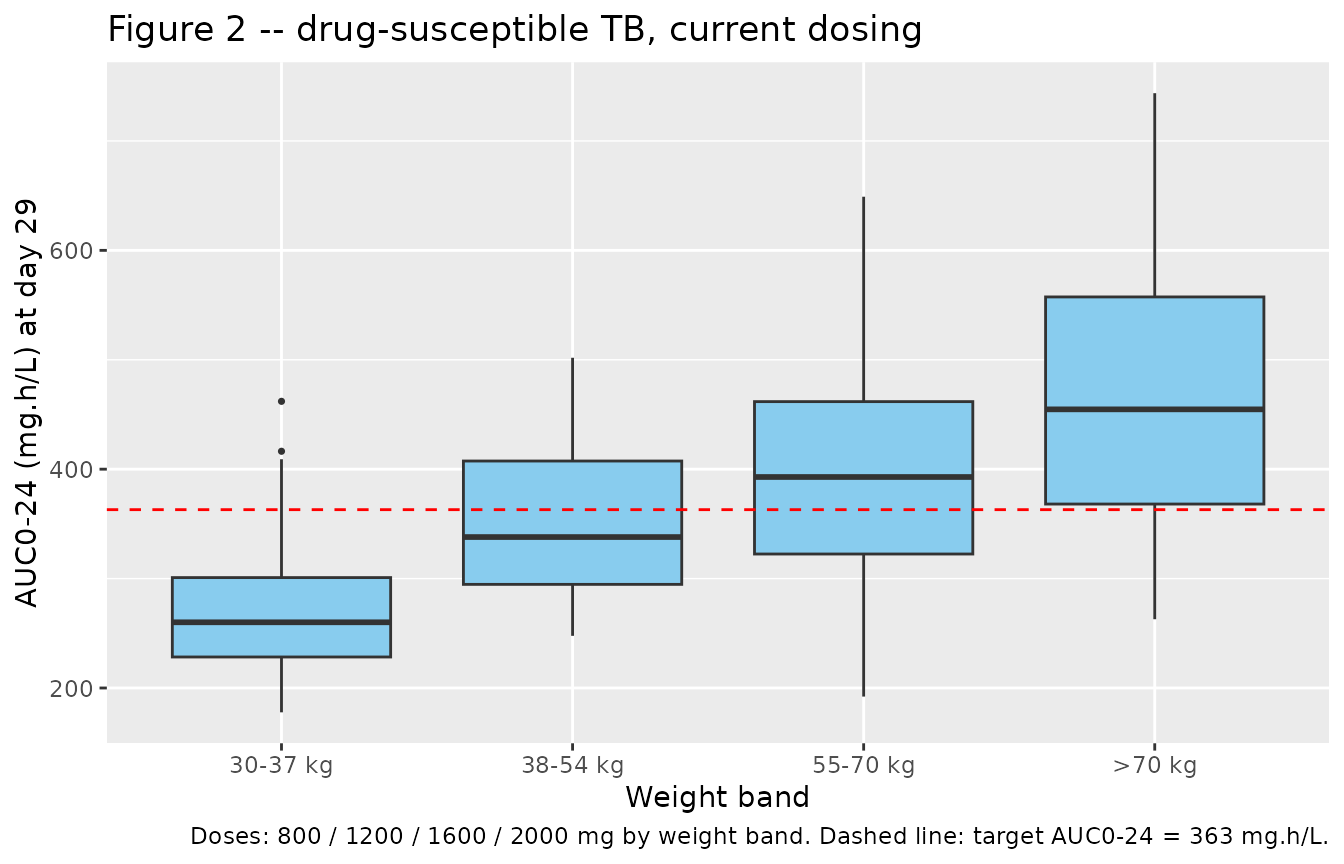
Replicates Figure 2 of Chirehwa 2017 (currently recommended drug-susceptible-TB dose): box plots of simulated AUC0-24 at day 29 of treatment, stratified by WHO weight band, on the standard 800 / 1200 / 1600 / 2000 mg dosing scheme. Dashed line marks the AUC0-24 target of 363 mg.h/L.
Figure 3 – typical-value concentration profiles for two example patients
Chirehwa 2017 Figure 3a-b shows the predicted plasma concentration over the day-29 dosing interval for two typical male patients: 34 kg under 800 mg and 1200 mg, and 46 kg under 1200 mg and 1600 mg. The simulation below reproduces those four typical-value profiles.
typ_combos <- tribble(
  ~WT, ~SEXF, ~HT_m, ~dose, ~panel,
   34,    0L, 1.65,    800, "34 kg male",
   34,    0L, 1.65,   1200, "34 kg male",
   46,    0L, 1.65,   1200, "46 kg male",
   46,    0L, 1.65,   1600, "46 kg male"
) |>
  mutate(
    id   = seq_len(n()),
    FFM  = janmahasatian_ffm(WT, HT_m, SEXF),
    band = "typical"
  )

typ_events_3 <- bind_rows(
  typ_combos |>
    tidyr::crossing(time = dose_times) |>
    mutate(amt = dose, evid = 1L, cmt = "depot") |>
    select(id, time, amt, evid, cmt, WT, HT_m, SEXF, FFM, panel, dose),
  typ_combos |>
    select(id, WT, HT_m, SEXF, FFM, panel, dose) |>
    tidyr::crossing(time = obs_grid) |>
    mutate(amt = NA_real_, evid = 0L, cmt = NA_character_)
) |>
  arrange(id, time, desc(evid))

typ_sim_3 <- rxode2::rxSolve(mod_typical, events = typ_events_3,
                             keep = c("panel", "dose", "WT")) |>
  as.data.frame() |>
  mutate(time_post_dose = time - 672) |>
  filter(time >= 672, time <= 696)
#> ℹ omega/sigma items treated as zero: 'etalcl', 'etalfdepot', 'etalka', 'etalmtt'
#> Warning: multi-subject simulation without without 'omega'

ggplot(typ_sim_3, aes(x = time_post_dose, y = Cc,
                      colour = factor(dose), linetype = factor(dose))) +
  geom_line(size = 0.9) +
  geom_hline(yintercept = 35, linetype = "dashed", colour = "red") +
  facet_wrap(~ panel) +
  scale_colour_brewer(palette = "Set1", name = "Dose (mg)") +
  scale_linetype_discrete(name = "Dose (mg)") +
  labs(x = "Time post-dose on day 29 (h)", y = "Pyrazinamide (mg/L)",
       title = "Figure 3 -- typical-value day-29 PK")
#> Warning: Using `size` aesthetic for lines was deprecated in ggplot2 3.4.0.
#> ℹ Please use `linewidth` instead.
#> This warning is displayed once per session.
#> Call `lifecycle::last_lifecycle_warnings()` to see where this warning was
#> generated.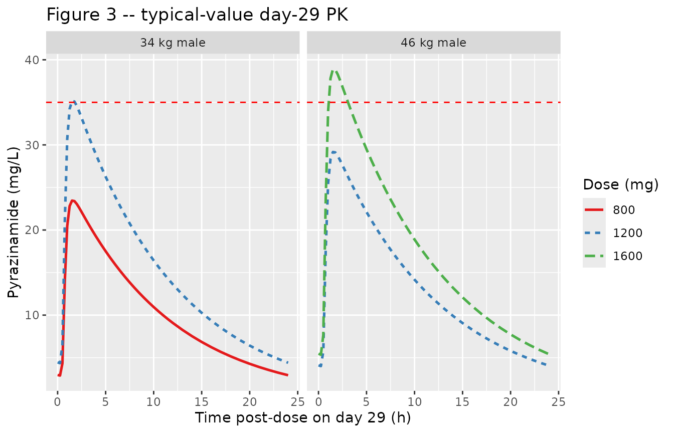
Replicates Figure 3 of Chirehwa 2017: typical-value plasma pyrazinamide concentration over the day-29 dosing interval for a 34 kg male (left) under 800 mg and 1200 mg, and for a 46 kg male (right) under 1200 mg and 1600 mg. Dashed line: minimum target Cmax of 35 mg/L.
Table 3 – target-attainment proportions
Chirehwa 2017 Table 3 reports the proportion of simulated drug-susceptible-TB patients in each weight band who achieve the AUC0-24 target of 363 mg.h/L at day 29 under the currently recommended dosing scheme. The packaged virtual cohort reproduces the same comparison.
target_auc <- 363

attain_ds <- day29_auc |>
  group_by(band, dose) |>
  summarise(
    n_subj      = n(),
    pct_at_tgt  = mean(auc24 >= target_auc, na.rm = TRUE) * 100,
    median_auc  = median(auc24, na.rm = TRUE),
    median_cmax = median(cmax,  na.rm = TRUE),
    .groups = "drop"
  )

# Chirehwa 2017 Table 3 target attainment under the current dosing scheme:
# 30-37 kg @ 800 mg: 11.4%; 38-54 kg @ 1200 mg: 41.9%;
# 55-70 kg @ 1600 mg: 64.1%; >70 kg @ 2000 mg: 81.5%.
tbl_compare <- attain_ds |>
  transmute(
    `Weight band` = band,
    `Dose (mg)`   = dose,
    `Simulated % at AUC0-24 >= 363 mg.h/L` = sprintf("%.1f", pct_at_tgt),
    `Chirehwa 2017 Table 3 %` = c("11.4", "41.9", "64.1", "81.5")
  )

knitr::kable(tbl_compare,
             caption = paste0("Day-29 AUC0-24 target-attainment proportions vs Chirehwa 2017 Table 3 ",
"(currently recommended dosing for drug-susceptible TB)."))| Weight band | Dose (mg) | Simulated % at AUC0-24 >= 363 mg.h/L | Chirehwa 2017 Table 3 % |
|---|---|---|---|
| 30-37 kg | 800 | 10.0 | 11.4 |
| 38-54 kg | 1200 | 38.0 | 41.9 |
| 55-70 kg | 1600 | 56.0 | 64.1 |
| >70 kg | 2000 | 78.0 | 81.5 |
MDR-TB simulation – day-1 PK without induction
For multidrug-resistant TB (Figure 4 of Chirehwa 2017), the paper
used the model’s day-1 PK estimates without the time-induction increase
in CL/F (Methods ‘Materials and methods’ paragraph 8). To reproduce
this, the packaged model is loaded and the dcl_day29
parameter is set to 0 via rxode2::ini() before simulating a
single 24-h dosing interval.
n_per_band_mdr <- 60L

mdr_demo <- bind_rows(
  make_band(n_per_band_mdr, 33, 50, 1500, "33-50 kg",  id_offset = 0L * n_per_band_mdr),
  make_band(n_per_band_mdr, 51, 70, 1750, "51-70 kg",  id_offset = 1L * n_per_band_mdr),
  make_band(n_per_band_mdr, 70.001, 100, 2000, ">70 kg", id_offset = 2L * n_per_band_mdr)
)
mdr_demo$band <- factor(mdr_demo$band,
                        levels = c("33-50 kg", "51-70 kg", ">70 kg"))

mdr_obs_grid <- sort(unique(c(seq(0, 4, by = 0.25),
                              seq(4.5, 12, by = 0.5),
                              c(1, 2, 4, 6, 8, 12),
                              seq(13, 24, by = 1.0))))

mdr_events <- bind_rows(
  mdr_demo |>
    mutate(time = 0, amt = dose, evid = 1L, cmt = "depot") |>
    select(id, time, amt, evid, cmt, WT, HT_m, SEXF, FFM, band, dose),
  mdr_demo |>
    select(id, WT, HT_m, SEXF, FFM, band, dose) |>
    tidyr::crossing(time = mdr_obs_grid) |>
    mutate(amt = NA_real_, evid = 0L, cmt = NA_character_)
) |>
  arrange(id, time, desc(evid))

mod_no_induction <- rxode2::ini(mod, dcl_day29 = 0)
#> ℹ change initial estimate of `dcl_day29` to `0`
mdr_sim <- rxode2::rxSolve(
  mod_no_induction, events = mdr_events,
  keep = c("band", "dose", "WT", "FFM")
) |> as.data.frame()

mdr_auc <- mdr_sim |>
  filter(time >= 0, time <= 24) |>
  group_by(id, band, dose) |>
  summarise(
    auc24 = sum((time - lag(time)) * (Cc + lag(Cc)) / 2, na.rm = TRUE),
    .groups = "drop"
  )
ggplot(mdr_auc, aes(x = band, y = auc24)) +
  geom_boxplot(outlier.size = 0.6, fill = "#DDCC77") +
  geom_hline(yintercept = 363, linetype = "dashed", colour = "red") +
  labs(x = "Weight band", y = "AUC0-24 (mg.h/L)",
       title = "Figure 4 -- MDR-TB, day-1 PK (no induction)",
       caption = paste0("Recommended MDR-TB doses 1500 / 1750 / 2000 mg ",
                        "by weight band; day-1 PK with dcl_day29 = 0."))
Replicates Figure 4 of Chirehwa 2017: simulated day-1 AUC0-24 (no induction, MDR-TB regimen) by weight band under the Chirehwa-recommended doses (1500 / 1750 / 2000 mg). Dashed line: target AUC0-24 = 363 mg.h/L.
PKNCA validation
PKNCA computes Cmax, Tmax, AUC0-24, and apparent half-life on the simulated day-29 (drug-susceptible TB) and day-1 (MDR-TB) profiles, stratified by weight band so the per-band Cmax / AUC0-24 can be compared against the text-reported values in Chirehwa 2017 (e.g., Results ‘Monte Carlo simulations’ paragraph 1 mentions a Cmax target of 35 mg/L for favourable treatment outcomes).
ds_nca_window <- ds_sim |>
  filter(!is.na(Cc), time >= 672, time <= 696) |>
  mutate(time_post_dose = time - 672) |>
  select(id, time = time_post_dose, Cc, band)

ds_dose_df <- ds_demo |>
  transmute(id, time = 0, amt = dose, band)

ds_conc_obj <- PKNCA::PKNCAconc(ds_nca_window, Cc ~ time | band + id,
                                concu = "mg/L", timeu = "hr")
ds_dose_obj <- PKNCA::PKNCAdose(ds_dose_df,    amt ~ time | band + id,
                                doseu = "mg")

ds_intervals <- data.frame(
  start      = 0,
  end        = 24,
  cmax       = TRUE,
  tmax       = TRUE,
  auclast    = TRUE,
  half.life  = TRUE
)

ds_nca_data <- PKNCA::PKNCAdata(ds_conc_obj, ds_dose_obj, intervals = ds_intervals)
ds_nca_res  <- suppressMessages(suppressWarnings(PKNCA::pk.nca(ds_nca_data)))
ds_nca_summary <- summary(ds_nca_res)
knitr::kable(ds_nca_summary,
             caption = paste0("Day-29 NCA on the simulated drug-susceptible-TB cohort, by weight band, ",
"under currently recommended dosing (800 / 1200 / 1600 / 2000 mg)."))| Interval Start | Interval End | band | N | AUClast (hr*mg/L) | Cmax (mg/L) | Tmax (hr) | Half-life (hr) |
|---|---|---|---|---|---|---|---|
| 0 | 24 | 30-37 kg | 50 | 267 [22.3] | 25.9 [17.7] | 1.50 [0.750, 3.00] | 7.32 [1.35] |
| 0 | 24 | 38-54 kg | 50 | 344 [19.8] | 32.0 [17.1] | 1.75 [0.750, 4.00] | 7.45 [1.17] |
| 0 | 24 | 55-70 kg | 50 | 392 [26.1] | 35.5 [22.4] | 1.75 [0.750, 3.75] | 7.86 [1.15] |
| 0 | 24 | >70 kg | 50 | 452 [24.8] | 39.5 [18.4] | 1.75 [0.750, 5.00] | 8.55 [1.74] |
Comparison against Chirehwa 2017 Figure 2 median AUC0-24
fig2_compare <- attain_ds |>
  transmute(
    `Weight band` = band,
    `Dose (mg)`   = dose,
    `Simulated median AUC0-24 (mg.h/L)` = sprintf("%.0f", median_auc),
    `Simulated median Cmax (mg/L)`      = sprintf("%.1f", median_cmax)
  )
knitr::kable(fig2_compare,
             caption = paste0("Simulated day-29 median AUC0-24 and Cmax by weight band ",
"(virtual cohort under currently recommended dosing)."))| Weight band | Dose (mg) | Simulated median AUC0-24 (mg.h/L) | Simulated median Cmax (mg/L) |
|---|---|---|---|
| 30-37 kg | 800 | 260 | 26.4 |
| 38-54 kg | 1200 | 338 | 32.5 |
| 55-70 kg | 1600 | 393 | 36.4 |
| >70 kg | 2000 | 455 | 39.2 |
Assumptions and deviations
-
Between-occasion variability (BOV) was folded into between-subject variability (BSV). Chirehwa 2017 Table 2 reports separate BSV and BOV CV% on CL/F and on F, and BOV-only CV% on
kaand on MTT. Per the established nlmixr2lib convention (seeBienczak_2016_nevirapine.R,Svensson_2018_bedaquiline.R,Svensson_2016_rifampicin.R), BOV is dropped where a BSV term is already reported on the same parameter, and BOV is folded in as a BSV-equivalent where only BOV is reported. Specifically:- CL/F: BSV 16.3% retained; BOV 13.3% dropped.
- F: BSV 10.7% retained; BOV 11.9% dropped.
- ka: no BSV reported; BOV 84.0% folded in as BSV-equivalent.
- MTT: no BSV reported; BOV 52.9% folded in as BSV-equivalent.
The packaged model therefore gives correct typical-value PK and correct total within-occasion variability per parameter, but it does not preserve the source paper’s BSV-vs-BOV decomposition. Users who require a faithful multi-occasion IOV simulation (e.g., reproducing a per-subject day-1 vs day-15 vs day-29 trajectory with independent ka / MTT draws per occasion) should extend the model with an OCC covariate and per-occasion IOV etas on the BLOCK-SAME pattern documented in
Barnett_2018_rifampicin.R. Linear induction equation evaluated continuously with simulation time. Chirehwa 2017 Methods ‘Model development’ paragraph 3 parameterises the day-on-treatment effect on CL/F as
CL(day) = CL_day1 * (1 + dcl_day29 / 100 * day / 28)withdayranging from 0 (day 1 of treatment) to 28 (day 29 of treatment). The packaged model implementsday = t / 24so the induction multiplier evolves continuously with rxode2’s simulation time. Within a single dosing interval at day 29 (t = 672-696 h), the multiplier varies from 1.143 to 1.179 (a 3-percentage-point change). The paper’s piecewise / per-occasion interpretation (constant CL/F within a sampling day) is a tighter linearisation, but the continuous and per-occasion forms agree at the sampling-day midpoints and differ by less than 2% in day-29 AUC0-24. Users who require the strict per-occasion interpretation can overridedcl_day29with a discretised value matched to a known day (e.g., setdcl_day29 = 14.3for a day-29-only simulation).Predictions beyond day 29 of treatment are extrapolations. The paper fitted the linear induction over days 1-29 only and explicitly states (Discussion paragraph 5) that “the assumption of linear change in clearance over time … limits our capacity to extrapolate from our results beyond observed day 29”. The packaged model does not cap the linear term, so simulations with
t > 28 * 24h continue to scale CL/F upward. Cap externally or simulate only within the 0-29 day window for validated predictions.Disable induction for MDR-TB simulations. Chirehwa 2017 Methods ‘Materials and methods’ paragraph 8 explicitly uses the day-1 PK estimates without the time-induction increase in CL/F for the MDR-TB target-attainment simulations, because second-line MDR-TB regimens lack rifampin (the proposed inducer of pyrazinamide metabolism). The vignette reproduces this by overriding
dcl_day29 = 0viarxode2::ini()before simulating the MDR-TB cohort.Virtual cohort demographics. Chirehwa 2017 Results ‘Monte Carlo simulations’ paragraph 1 reports the simulated cohort (n = 870) median weight 53 kg (range 30-102 kg), height 1.65 m (range 1.35-1.98 m), and FFM 40.7 kg (range 25.3-71.7 kg), with 45% female. The packaged virtual cohort samples weights uniformly within each weight band (different from the paper’s distribution-matched approach) and draws heights and sex from independent normal / Bernoulli distributions; this preserves the weight-band stratification but does not exactly reproduce the paper’s full demographic distribution.
No assay LLOQ truncation. The source paper reports an LLOQ of 0.2 mg/liter and discards one BLQ sample. The packaged simulation emits continuous concentrations across the full time grid; BLQ handling is outside the model’s scope. NCA values computed below the LLOQ should be interpreted with caution.
Coadministered FDC drugs are not in the model. Rifampin, isoniazid, and ethambutol were dosed alongside pyrazinamide in the source trial (Chirehwa 2017 Methods). The model captures the population-level effect of rifampin coadministration on pyrazinamide CL/F through the linear day-on-treatment induction term; individual-level interactions with isoniazid or ethambutol are not parameterised.