Batiraxcept (Bonifacio 2020)
Source:vignettes/articles/Bonifacio_2020_batiraxcept.Rmd
Bonifacio_2020_batiraxcept.RmdModel and source
- Citation: Bonifacio L, Dodds M, Prohaska D, Moss A, Giaccia A, Tabibiazar R, McIntyre G. (2020). Target-Mediated Drug Disposition Pharmacokinetic/Pharmacodynamic Model-Informed Dose Selection for the First-in-Human Study of AVB-S6-500. Clinical and Translational Science 13(1), 204-211. doi:10.1111/cts.12706. Model equations and the PD parameter table are in Supplementary Material CTS-13-204-s001.docx.
- Description: Preclinical (cynomolgus monkey), allometrically scaled to human. Two-compartment population PK model for batiraxcept (AVB-S6-500, an AXL-ectodomain / IgG1 Fc fusion protein that neutralises GAS6) with parallel linear and Michaelis-Menten (target-mediated) elimination from the central compartment, fit to cynomolgus monkey serum concentrations (0.1-150 mg/kg) with parameters centred on a 70 kg subject. CL, Q and Vmax scale with (WT/70)^0.75 and VC, VP with (WT/70)^1. A direct (no-hysteresis) inhibitory sigmoid Emax relationship drives serum free GAS6 suppression from the drug concentration (not scaled between species). The paper used the typical-value model to select the first-in-human doses (1, 2.5, 5, 10 mg/kg IV) in healthy volunteers.
- Article: https://doi.org/10.1111/cts.12706 (open access, PMC6951457)
- Supplement: Supplementary Material
CTS-13-204-s001.docx(model equations, PK and PD parameter tables, monkey VPCs)
Batiraxcept (AVB-S6-500) is a fusion of the AXL extracellular domain and a human IgG1 Fc that binds growth arrest-specific 6 (GAS6) protein with femtomolar affinity. Bonifacio 2020 fit a two-compartment model with parallel linear and Michaelis-Menten (target-mediated) elimination to cynomolgus monkey serum concentrations, scaled it allometrically to humans, and linked the serum drug concentration to serum free GAS6 through a direct inhibitory sigmoid Emax relationship. The typical-value human projection was used to pick the first-in-human (FIH) doses, and the FIH study served as an external validation.
Population
The model was fit to data from five nonclinical cynomolgus monkey studies covering 0.1 to 150 mg/kg: 2 animals per dose level at 0.1, 0.5 and 1 mg/kg, 4 animals at 5 mg/kg (two studies), 12 animals per dose level over 30-100 mg/kg (three studies) and 18 animals at 150 mg/kg (Methods, “Nonclinical studies used for PK/PD model development”). The total animal count and the animal body weights are not reported. PK parameters are reported centred on a 70 kg subject.
The external validation cohort (NCT03401528; Table 1) was 31 healthy volunteers receiving batiraxcept by 60-minute IV infusion: single doses of 1, 2.5, 5 or 10 mg/kg (6 per group) or 5 mg/kg once weekly for 4 weeks (7), aged 22-54 years, median weight 75.5 kg, predominantly Black or African American and male. The paper’s pre-study simulations used a 75 kg typical subject; this vignette does the same.
The same information is available programmatically via
readModelDb("Bonifacio_2020_batiraxcept")()$population.
Source trace
| Equation / parameter | Value | Source location |
|---|---|---|
lcl (CL at 70 kg) |
1.10 L/day | Table 2; Supplement Table 1 |
lvc (VC at 70 kg) |
2.97 L | Table 2; Supplement Table 1 |
lvp (VP at 70 kg) |
2.94 L | Table 2; Supplement Table 1 |
lq (Q at 70 kg) |
2.04 L/day | Table 2; Supplement Table 1 |
lvmax (Vmax at 70 kg) |
3.35 mg/day | Table 2; Supplement Table 1 |
lkm (KM) |
102 ng/mL = 0.102 ug/mL | Table 2; Supplement Table 1 |
e_wt_cl |
0.75 (not estimated) | Methods “Model predictions of clinical PK/PD”; Supplement “Scaling to Human Pharmacokinetics” |
e_wt_vc |
1.0 (not estimated) | Same as above |
lrbase (E0, baseline GAS6) |
23.8 ng/mL | Supplement Table 2 |
lec50 (EC50) |
21.4 ng/mL = 0.0214 ug/mL | Supplement Table 2 |
lhill (H) |
0.796 | Supplement Table 2 |
etalcl, etalvc, etalvp,
etalq, etalvmax, etalkm
|
29.7, 14.0, 14.3, 50.0, 98.6, 103 CV% -> omega^2 = log(CV^2 + 1) | Table 2; Supplement Table 1 |
propSd |
proportional; magnitude not reported, encoded
fixed(0)
|
Supplement “Non-Human Primate Pharmacokinetic Analysis” |
d/dt(central), d/dt(peripheral1)
|
two-compartment with parallel linear + Michaelis-Menten loss of
Ap
|
Supplement Methods (dAp/dt, dAt/dt); Figure 1 |
GAS6 <- E0 * (1 - C^H / (EC50^H + C^H)) |
direct effect | Supplement “Non-Human Primate Pharmacodynamic Analysis” |
Allometric scaling (WT/70)^0.75 on CL, Q, Vmax;
(WT/70)^1 on VC, VP |
Supplement “Scaling to Human Pharmacokinetics” |
Typical-subject simulation of the FIH regimens
The paper’s human projections (Figures 2 and 3, Table 3) are typical-value predictions for a 75 kg subject; between-animal variability was deliberately not propagated (Supplement Results; Discussion). The random effects are therefore zeroed here.
wt_sim <- 75
inf_dur <- 1 / 24 # 60-minute infusion, in days

regimens <- tibble::tribble(
  ~treatment,           ~dose_mgkg, ~n_doses,
  "1 mg/kg",            1,          1L,
  "2.5 mg/kg",          2.5,        1L,
  "5 mg/kg",            5,          1L,
  "10 mg/kg",           10,         1L,
  "5 mg/kg q.w. x 4",   5,          4L
)

obs_times <- sort(unique(c(
  seq(0, 63, by = 1 / 24),
  inf_dur + 7 * (0:3)
)))

make_regimen <- function(i) {
  r <- regimens[i, ]
  dose_times <- 7 * (seq_len(r$n_doses) - 1)
  doses <- tibble(
    id = i, time = dose_times, evid = 1L, amt = r$dose_mgkg * wt_sim,
    rate = r$dose_mgkg * wt_sim / inf_dur, cmt = "central"
  )
  obs <- tibble(
    id = i, time = obs_times, evid = 0L, amt = 0, rate = 0, cmt = "central"
  )
  bind_rows(doses, obs) |>
    mutate(treatment = r$treatment, WT = wt_sim) |>
    arrange(time, desc(evid))
}

events_typ <- bind_rows(lapply(seq_len(nrow(regimens)), make_regimen))
stopifnot(!anyDuplicated(events_typ[, c("id", "time", "evid")]))
mod <- readModelDb("Bonifacio_2020_batiraxcept")
mod_typ <- rxode2::zeroRe(mod)
#> ℹ parameter labels from comments will be replaced by 'label()'
sim_typ <- rxode2::rxSolve(
  mod_typ,
  events = events_typ, keep = c("treatment"),
  rtol = 1e-10, atol = 1e-12
) |>
  as.data.frame() |>
  mutate(treatment = factor(treatment, levels = regimens$treatment))
#> ℹ omega/sigma items treated as zero: 'etalcl', 'etalvc', 'etalvp', 'etalq', 'etalvmax', 'etalkm'
#> Warning: multi-subject simulation without without 'omega'
Figure 2: serum batiraxcept
# Replicates the model lines of Figure 2 of Bonifacio 2020 (typical 75 kg
# subject). LLOQ 10 ng/mL = 0.01 ug/mL; values below LLOQ plotted at LLOQ/2
# as in the paper.
lloq_pk <- 0.01
sim_typ |>
  filter(time > 0) |>
  mutate(Cc_plot = ifelse(Cc < lloq_pk, lloq_pk / 2, Cc)) |>
  ggplot(aes(time, Cc_plot)) +
  geom_line(colour = "steelblue") +
  geom_hline(yintercept = lloq_pk, linetype = "dashed", colour = "red") +
  facet_wrap(~treatment) +
  scale_y_log10() +
  labs(
    x = "Time (day)", y = "Batiraxcept (ug/mL)",
    caption = "Replicates the typical-subject predictions of Figure 2 of Bonifacio 2020."
  )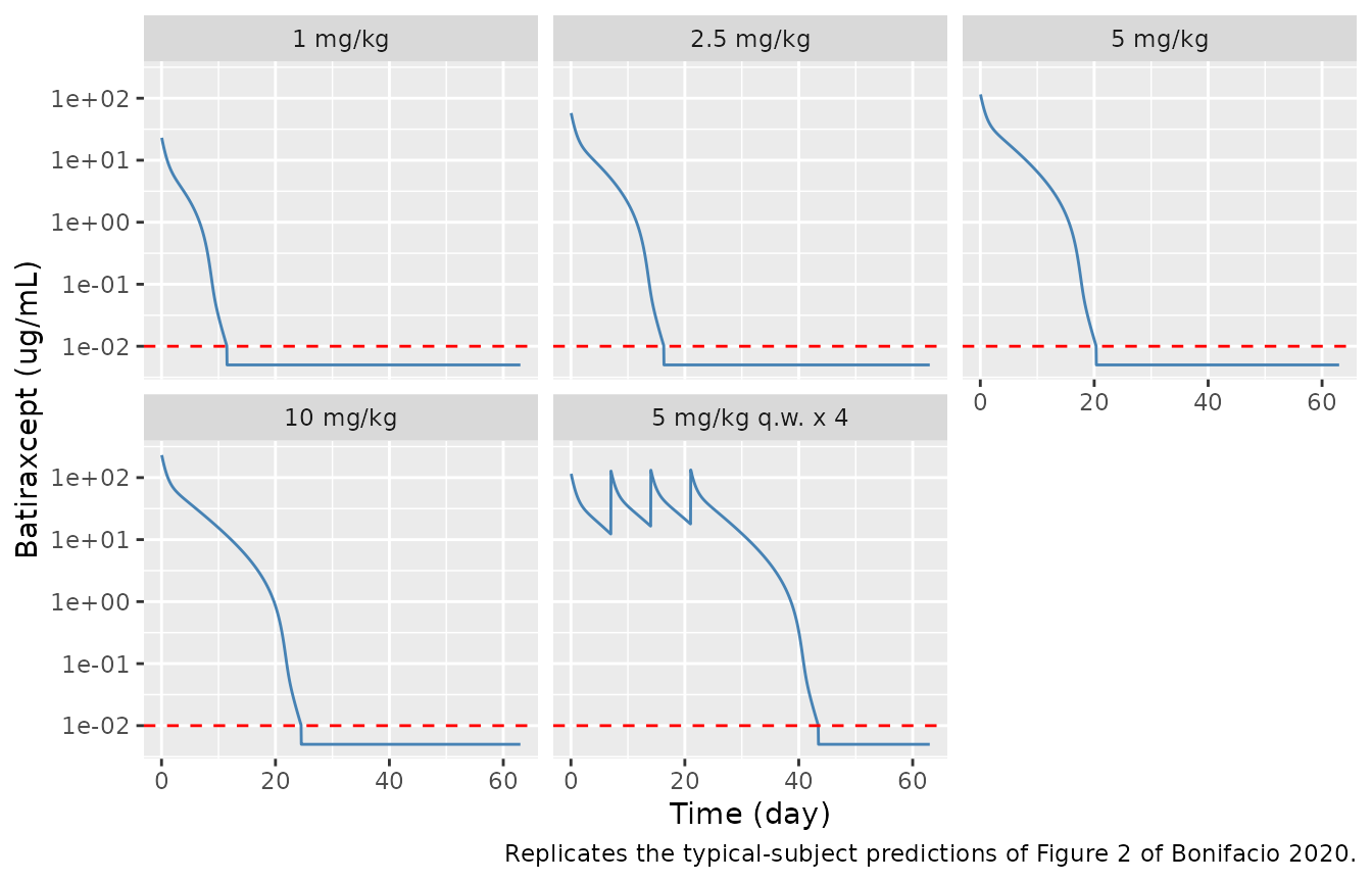
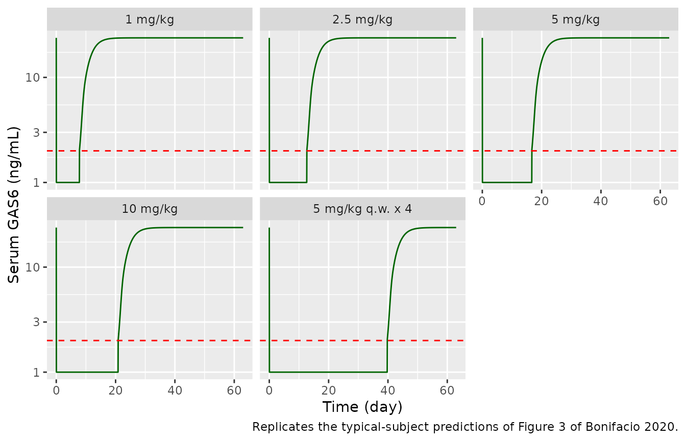
Figure 3: serum GAS6
# Replicates the model lines of Figure 3 of Bonifacio 2020. GAS6 LLOQ in the
# FIH study was 2 ng/mL; values below LLOQ plotted at LLOQ/2.
lloq_gas6 <- 2
sim_typ |>
  mutate(GAS6_plot = ifelse(GAS6 < lloq_gas6, lloq_gas6 / 2, GAS6)) |>
  ggplot(aes(time, GAS6_plot)) +
  geom_line(colour = "darkgreen") +
  geom_hline(yintercept = lloq_gas6, linetype = "dashed", colour = "red") +
  facet_wrap(~treatment) +
  scale_y_log10() +
  labs(
    x = "Time (day)", y = "Serum GAS6 (ng/mL)",
    caption = "Replicates the typical-subject predictions of Figure 3 of Bonifacio 2020."
  )
PKNCA validation against Table 3 (model-predicted values)
Table 3 of Bonifacio 2020 lists the model-predicted Cmax and AUC0-tau for the typical 75 kg subject next to the observed FIH values. The predicted column is the direct reproduction target for this model; the observed column is an external comparison that the paper itself reports as underpredicted for AUC (44.6-72.4% predicted/observed). AUC0-tau is computed over one week (0-7 days for the single doses and the first weekly dose, 21-28 days for the fourth weekly dose), which is the interval that reproduces the paper’s predicted values. Model time is in days, so the published ug*h/mL values are divided by 24.
conc_df <- sim_typ |>
  filter(!is.na(Cc)) |>
  mutate(Cc = pmax(Cc, 0)) |>
  select(id, time, Cc, treatment) |>
  mutate(treatment = as.character(treatment))

dose_df <- events_typ |>
  filter(evid == 1) |>
  select(id, time, amt, treatment)

conc_obj <- PKNCA::PKNCAconc(conc_df, Cc ~ time | treatment + id)
dose_obj <- PKNCA::PKNCAdose(dose_df, amt ~ time | treatment + id)

intervals <- bind_rows(
  data.frame(
    treatment = regimens$treatment, start = 0, end = 7,
    cmax = TRUE, auclast = TRUE
  ),
  data.frame(
    treatment = "5 mg/kg q.w. x 4", start = 21, end = 28,
    cmax = TRUE, auclast = TRUE
  )
)

nca_res <- PKNCA::pk.nca(
  PKNCA::PKNCAdata(conc_obj, dose_obj, intervals = intervals)
)

sim_nca <- as.data.frame(nca_res$result) |>
  mutate(
    group = case_when(
      treatment == "5 mg/kg q.w. x 4" & start == 0 ~ "5 mg/kg q.w. x 4, dose 1",
      treatment == "5 mg/kg q.w. x 4" & start == 21 ~ "5 mg/kg q.w. x 4, dose 4",
      TRUE ~ treatment
    )
  ) |>
  select(group, PPTESTCD, PPORRES)

# Table 3, predicted values (Cmax ug/mL; AUC0-tau ug*h/mL converted to ug*day/mL)
published <- tibble::tribble(
  ~group,                      ~cmax, ~auclast,
  "1 mg/kg",                   23.2,  869 / 24,
  "2.5 mg/kg",                 58.2,  2520 / 24,
  "5 mg/kg",                   116,   5290 / 24,
  "10 mg/kg",                  233,   10800 / 24,
  "5 mg/kg q.w. x 4, dose 1",  116,   5290 / 24,
  "5 mg/kg q.w. x 4, dose 4",  134,   7060 / 24
)

cmp <- nlmixr2lib::ncaComparisonTable(
  simulated = sim_nca,
  reference = published,
  by = "group",
  units = c(cmax = "ug/mL", auclast = "ug*day/mL"),
  tolerance_pct = 20
)
knitr::kable(
  cmp,
  digits = 2,
  caption = "Simulated typical-subject NCA vs. Bonifacio 2020 Table 3 model-predicted values. * differs by >20%."
)| NCA parameter | group | Reference | Simulated | % diff |
|---|---|---|---|---|
| Cmax (ug/mL) | 1 mg/kg | 23.2 | 23 | -0.8% |
| Cmax (ug/mL) | 2.5 mg/kg | 58.2 | 57.6 | -1.0% |
| Cmax (ug/mL) | 5 mg/kg | 116 | 115 | -0.6% |
| Cmax (ug/mL) | 10 mg/kg | 233 | 231 | -1.0% |
| Cmax (ug/mL) | 5 mg/kg q.w. x 4, dose 1 | 116 | 115 | -0.6% |
| Cmax (ug/mL) | 5 mg/kg q.w. x 4, dose 4 | 134 | 133 | -0.7% |
| AUClast (ug*day/mL) | 1 mg/kg | 36.2 | 36.7 | +1.4% |
| AUClast (ug*day/mL) | 2.5 mg/kg | 105 | 106 | +1.2% |
| AUClast (ug*day/mL) | 5 mg/kg | 220 | 223 | +1.0% |
| AUClast (ug*day/mL) | 10 mg/kg | 450 | 455 | +1.1% |
| AUClast (ug*day/mL) | 5 mg/kg q.w. x 4, dose 1 | 220 | 223 | +1.0% |
| AUClast (ug*day/mL) | 5 mg/kg q.w. x 4, dose 4 | 294 | 300 | +1.8% |
chk <- sim_nca |>
  inner_join(
    published |> pivot_longer(-group, names_to = "PPTESTCD", values_to = "ref"),
    by = c("group", "PPTESTCD")
  ) |>
  mutate(pct_diff = 100 * (PPORRES / ref - 1))
knitr::kable(chk, digits = 2)| group | PPTESTCD | PPORRES | ref | pct_diff |
|---|---|---|---|---|
| 1 mg/kg | auclast | 36.71 | 36.21 | 1.39 |
| 1 mg/kg | cmax | 23.02 | 23.20 | -0.75 |
| 2.5 mg/kg | auclast | 106.30 | 105.00 | 1.23 |
| 2.5 mg/kg | cmax | 57.63 | 58.20 | -0.98 |
| 5 mg/kg | auclast | 222.52 | 220.42 | 0.96 |
| 5 mg/kg | cmax | 115.30 | 116.00 | -0.60 |
| 10 mg/kg | auclast | 455.04 | 450.00 | 1.12 |
| 10 mg/kg | cmax | 230.65 | 233.00 | -1.01 |
| 5 mg/kg q.w. x 4, dose 1 | auclast | 222.52 | 220.42 | 0.96 |
| 5 mg/kg q.w. x 4, dose 1 | cmax | 115.30 | 116.00 | -0.60 |
| 5 mg/kg q.w. x 4, dose 4 | auclast | 299.61 | 294.17 | 1.85 |
| 5 mg/kg q.w. x 4, dose 4 | cmax | 133.08 | 134.00 | -0.68 |
# Both sides are typical-value predictions of the same model, so the only
# differences are the paper's rounding and its (unreported) output grid and
# integration. Measured: Cmax -0.6% to -1.0%, AUC +1.0% to +1.9%. A 5% bound
# still fails on any mis-transcribed volume, clearance, Vmax or unit, each of
# which moves these values by tens of percent.
stopifnot(nrow(chk) == 12L, all(abs(chk$pct_diff) < 5))
GAS6 suppression versus the paper’s narrative
The Results describe the typical-subject GAS6 prediction qualitatively at each follow-up visit (GAS6 LLOQ 2 ng/mL, baseline 23.8 ng/mL). The table below shows the simulated typical GAS6 at those visits.
gas6_visits <- sim_typ |>
  filter(treatment != "5 mg/kg q.w. x 4", abs(time - round(time)) < 1e-6, round(time) %in% c(7, 14, 21, 28)) |>
  mutate(time = round(time)) |>
  select(treatment, time, Cc, GAS6) |>
  mutate(pct_of_baseline = 100 * GAS6 / 23.8)
knitr::kable(gas6_visits, digits = 3)| treatment | time | Cc | GAS6 | pct_of_baseline |
|---|---|---|---|---|
| 1 mg/kg | 7 | 0.820 | 1.239 | 5.204 |
| 1 mg/kg | 14 | 0.002 | 20.838 | 87.556 |
| 1 mg/kg | 21 | 0.000 | 23.707 | 99.608 |
| 1 mg/kg | 28 | 0.000 | 23.797 | 99.989 |
| 2.5 mg/kg | 7 | 5.081 | 0.302 | 1.269 |
| 2.5 mg/kg | 14 | 0.073 | 6.524 | 27.411 |
| 2.5 mg/kg | 21 | 0.000 | 22.733 | 95.515 |
| 2.5 mg/kg | 28 | 0.000 | 23.769 | 99.869 |
| 5 mg/kg | 7 | 12.311 | 0.150 | 0.631 |
| 5 mg/kg | 14 | 2.060 | 0.612 | 2.569 |
| 5 mg/kg | 21 | 0.006 | 17.225 | 72.376 |
| 5 mg/kg | 28 | 0.000 | 23.559 | 98.986 |
| 10 mg/kg | 7 | 26.795 | 0.081 | 0.341 |
| 10 mg/kg | 14 | 6.784 | 0.241 | 1.011 |
| 10 mg/kg | 21 | 0.371 | 2.225 | 9.348 |
| 10 mg/kg | 28 | 0.001 | 21.890 | 91.976 |
g <- function(trt, day) gas6_visits$GAS6[gas6_visits$treatment == trt & gas6_visits$time == day]
stopifnot(
  # "undetectable" at day 7 for every single dose, and at day 14 for 5 and
  # 10 mg/kg (paper Results).
  g("1 mg/kg", 7) < lloq_gas6,
  g("2.5 mg/kg", 7) < lloq_gas6,
  g("5 mg/kg", 14) < lloq_gas6,
  g("10 mg/kg", 14) < lloq_gas6,
  # "nearly baseline" at day 14 for 1 mg/kg and day 21 for 5 mg/kg, and at
  # day 28 for 10 mg/kg (above half of baseline).
  g("1 mg/kg", 14) > 0.5 * 23.8,
  g("5 mg/kg", 21) > 0.5 * 23.8,
  g("10 mg/kg", 28) > 0.5 * 23.8,
  # "just-detectable" at day 14 for 2.5 mg/kg and day 21 for 10 mg/kg: above
  # the LLOQ but well below baseline.
  g("2.5 mg/kg", 14) > lloq_gas6, g("2.5 mg/kg", 14) < 0.5 * 23.8,
  g("10 mg/kg", 21) > lloq_gas6, g("10 mg/kg", 21) < 0.5 * 23.8
)
The Supplement also states that batiraxcept concentrations above ~2000 ng/mL suppress GAS6 below the monkey assay LLOQ of 0.78 ng/mL, and that a concentration at the 10 ng/mL PK LLOQ corresponds to at least 50% suppression. Checking both against the PD equation:
pd <- function(C) 23.8 * (1 - C^0.796 / (0.0214^0.796 + C^0.796))
c(GAS6_at_2_ug_per_mL = pd(2), GAS6_at_0.01_ug_per_mL = pd(0.01))
#>    GAS6_at_2_ug_per_mL GAS6_at_0.01_ug_per_mL
#>               0.625742              15.397095
stopifnot(pd(2) < 0.78)
With the printed estimates, GAS6 at 2 ug/mL is below the 0.78 ng/mL monkey LLOQ, as stated. At the 10 ng/mL PK LLOQ, however, GAS6 is only 35% suppressed, not “at least 50%”: EC50 (21.4 ng/mL) is above the PK LLOQ, so 50% suppression is reached only at 21.4 ng/mL. This is an approximation in the paper’s wording and was not tuned.
Between-subject variability (illustration)
The paper states that, at low doses, the TMDD variability (Vmax and KM CV ~100%) produces a wide prediction interval while at 5-10 mg/kg the pathway is saturated and variability matters less. The between-animal variances are packaged for completeness, but the authors note they have no known relationship to human variability and did not use them for human projections. The simulation below (200 virtual 75 kg subjects per dose, single dose, no residual error because its magnitude was not reported) illustrates the statement.
rxode2::rxSetSeed(20200101)
bsv_regs <- regimens |> filter(n_doses == 1L)
events_bsv <- bind_rows(lapply(seq_len(nrow(bsv_regs)), function(i) {
  r <- bsv_regs[i, ]
  ids <- (i - 1L) * 200L + seq_len(200L)
  d <- tibble(
    id = ids, time = 0, evid = 1L, amt = r$dose_mgkg * wt_sim,
    rate = r$dose_mgkg * wt_sim / inf_dur, cmt = "central"
  )
  o <- tidyr::expand_grid(id = ids, time = seq(0, 28, by = 0.25)) |>
    mutate(evid = 0L, amt = 0, rate = 0, cmt = "central")
  bind_rows(d, o) |>
    mutate(treatment = r$treatment, WT = wt_sim) |>
    arrange(id, time, desc(evid))
}))
stopifnot(!anyDuplicated(events_bsv[, c("id", "time", "evid")]))

sim_bsv <- rxode2::rxSolve(mod, events = events_bsv, keep = "treatment") |>
  as.data.frame() |>
  mutate(treatment = factor(treatment, levels = bsv_regs$treatment))
#> ℹ parameter labels from comments will be replaced by 'label()'

sim_bsv |>
  filter(time > 0) |>
  group_by(treatment, time) |>
  summarise(
    Q05 = quantile(Cc, 0.05), Q50 = median(Cc), Q95 = quantile(Cc, 0.95),
    .groups = "drop"
  ) |>
  ggplot(aes(time, Q50)) +
  geom_ribbon(aes(ymin = pmax(Q05, 1e-3), ymax = Q95), alpha = 0.25, fill = "steelblue") +
  geom_line(colour = "steelblue") +
  geom_hline(yintercept = lloq_pk, linetype = "dashed", colour = "red") +
  facet_wrap(~treatment) +
  scale_y_log10() +
  labs(
    x = "Time (day)", y = "Batiraxcept (ug/mL)",
    caption = "Median and 90% interval, between-animal variability applied to 75 kg subjects (illustrative)."
  )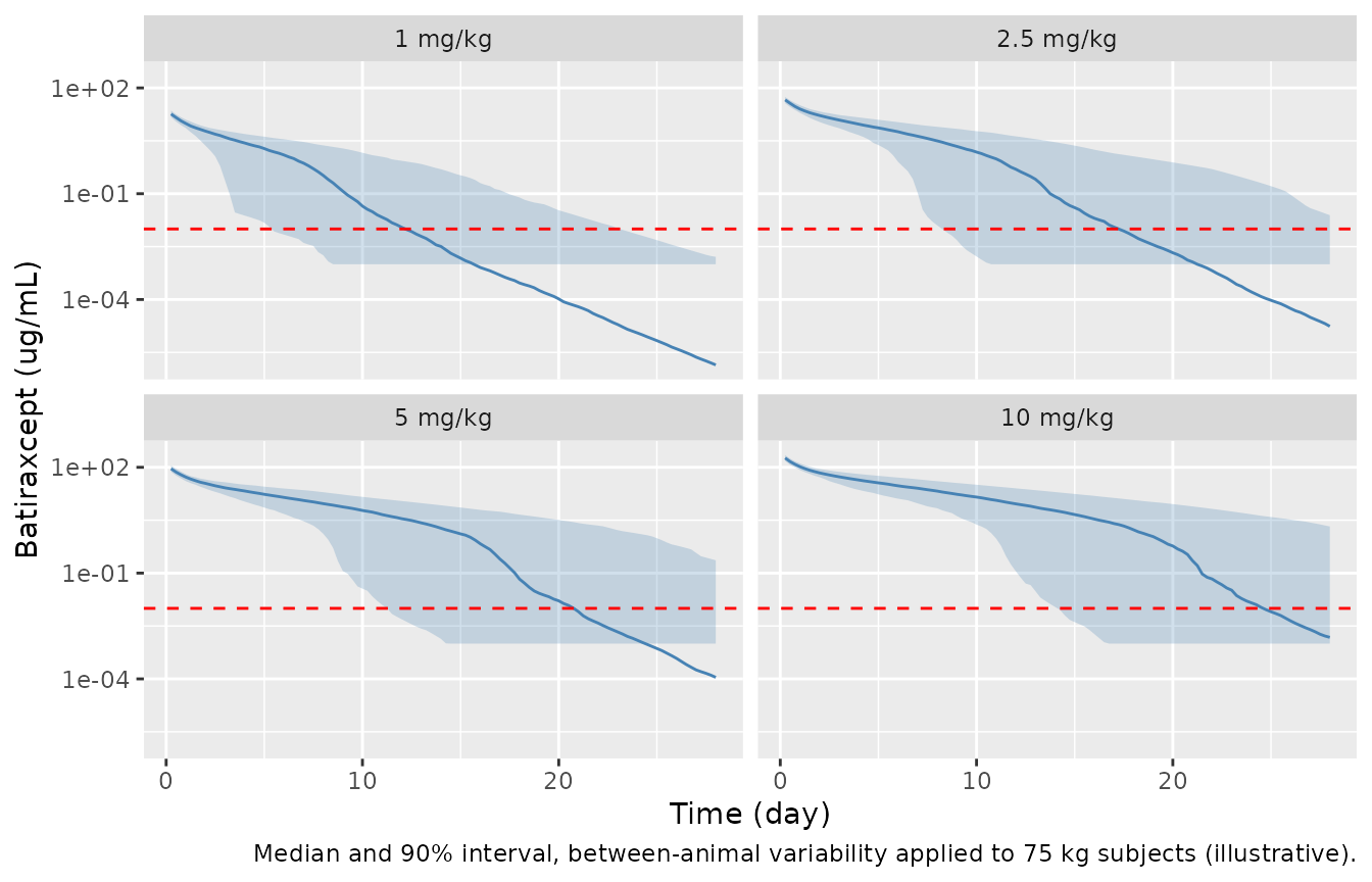
spread <- sim_bsv |>
  filter(abs(time - 14) < 1e-6) |>
  group_by(treatment) |>
  summarise(
    frac_below_lloq = mean(Cc < lloq_pk),
    iqr_log10 = diff(quantile(log10(pmax(Cc, 1e-6)), c(0.25, 0.75))),
    .groups = "drop"
  )
knitr::kable(spread, digits = 2)| treatment | frac_below_lloq | iqr_log10 |
|---|---|---|
| 1 mg/kg | 0.64 | 1.99 |
| 2.5 mg/kg | 0.30 | 2.30 |
| 5 mg/kg | 0.19 | 2.27 |
| 10 mg/kg | 0.05 | 0.71 |
Assumptions and deviations
- Drug name. The paper refers only to the development code AVB-S6-500; the file uses the INN batiraxcept.
-
Residual error. The Supplement states that residual
variability was proportional but does not report its magnitude (in
either the main text or the Supplement), so
propSdis encoded asfixed(0). Simulations with residual error need a user-supplied value. - Omega scale and covariances. Between-animal variability is reported as CV%; it was converted with omega^2 = log(CV^2 + 1) (the paper does not state which CV convention it used). The Supplement says “variance terms were modeled with variance-covariance interactions” but the covariances are not reported, so a diagonal omega is used. These variances describe monkeys and were not used by the authors for human projections.
-
PD model. The GAS6 Emax model was fit separately
(Supplement Table 2 reports estimate / SE / statistic / p-value, i.e. a
regression fit, not a joint NONMEM fit), with no residual-error or
between-subject variability reported. It is packaged as the algebraic
output
GAS6(ng/mL) driven byCc(ug/mL; EC50 converted from 21.4 ng/mL) and carries no error model. No interspecies scaling was applied to the PD (paper Methods), so E0 is the monkey baseline (23.8 ng/mL). - LLOQ statements. The Supplement’s “PK LLOQ implies at least 50% suppression” does not hold exactly with the printed EC50 (see above); this is recorded, not tuned.
- External validation. Observed FIH Cmax and AUC (Table 3) are not gated: the paper reports AUC predicted/observed of 44.6-72.4%, i.e. the model (as published) underpredicts human exposure at later times.
- Monkey population. Animal weights and the total animal count are not reported, so the monkey fit cannot be re-simulated at animal-level covariates; the monkey VPCs (Supplement Figures 2 and 3) are not reproduced.