Fosdagrocorat (Weatherley 2018)
Source:vignettes/articles/Weatherley_2018_fosdagrocorat.Rmd
Weatherley_2018_fosdagrocorat.RmdModel and source
- Citation: Weatherley B, McFadyen L, Tammara B. Population pharmacokinetics of fosdagrocorat (PF-04171327), a dissociated glucocorticoid receptor agonist, in patients with rheumatoid arthritis. Clin Transl Sci. 2018;11(1):54-62. doi:10.1111/cts.12515
- Article: https://doi.org/10.1111/cts.12515
- Open-access full text (Wiley): https://ascpt.onlinelibrary.wiley.com/doi/10.1111/cts.12515
The packaged model is Weatherley_2018_fosdagrocorat.
Fosdagrocorat is a phosphate-ester prodrug that is cleaved by alkaline
phosphatase in the gut wall, yielding the active dissociated
glucocorticoid receptor agonist PF-00251802 (“Metabolite-1”);
Metabolite-1 is in turn oxidised to the circulating N-oxide PF-04015475
(“Metabolite-2”). The model fits Metabolite-1 to a two-compartment
disposition (central V2, peripheral V4 fixed at 209 L) with first-order
absorption (K12); the fractions of prodrug-to-Metabolite-1 and
Metabolite-1-to-Metabolite-2 conversion are both fixed at unity
(apparent F absorbs the prodrug cleavage and the molar conversion).
Metabolite-2 is described by a one-compartment disposition (Vm,
CLm).
Population
The popPK dataset comprised 1607 Metabolite-1 and 1607 Metabolite-2 plasma concentrations from 179 adult rheumatoid-arthritis patients enrolled in study A9391010 (NCT01393639), a 12-week phase II randomised double-blind dose-ranging study (Weatherley 2018 Table 1):
- Patients were randomised 1:1:1:1:1:1:1 to fosdagrocorat 1, 5, 10, or 15 mg once daily, prednisone 5 or 10 mg once daily, or matched placebo. Only the four fosdagrocorat arms (179 patients) were modelled for Metabolite-1 and Metabolite-2.
- 76 percent of patients were female (Weatherley 2018 Table 1 by-arm counts: 32 / 36 / 34 / 34 in the 1, 5, 10, 15 mg arms).
- Mean body weight was approximately 80 kg in male patients and 73 kg in female patients (Table 1 by-arm means with SDs 14-23 kg).
- Mean age was 53 years (range 18-84 across the cohorts).
- Baseline creatinine clearance was approximately 100-130 mL/min on average; creatinine clearance was tested as a covariate on Metabolite-1 CL and Metabolite-2 CLm but was not retained in the final model.
The same metadata is available programmatically:
nlmixr2lib::readModelDb("Weatherley_2018_fosdagrocorat")$populationSource trace
Per-parameter origin is recorded inline next to each
ini() entry in
inst/modeldb/specificDrugs/Weatherley_2018_fosdagrocorat.R.
The table below collects the same provenance for review.
| Equation / parameter | Value | Source location |
|---|---|---|
lka (= K12) |
log(0.377 1/h) | Weatherley 2018 Table 2 ‘Without BLQ or taper’ |
lcl (Metabolite-1 CL) |
log(7.29 L/h) | Weatherley 2018 Table 2 |
lvc (Metabolite-1 V2) |
log(85.9 L) | Weatherley 2018 Table 2 |
lq (Metabolite-1 Q) |
log(11.6 L/h) | Weatherley 2018 Table 2 |
lvp (Metabolite-1 V4, fixed) |
log(209 L) | Weatherley 2018 Table 2 + Results page 58 |
lfdepot (F1, fixed) |
log(1) | Weatherley 2018 Table 2 |
lcl_noxide (Metabolite-2 CLm) |
log(17.2 L/h) | Weatherley 2018 Table 2 |
lvc_noxide (Metabolite-2 Vm) |
log(62.8 L) | Weatherley 2018 Table 2 |
e_wt_cl / e_wt_q (allometric
exponents) |
0.75 fixed | Weatherley 2018 Results page 58 |
e_wt_vc / e_wt_vp (allometric
exponents) |
1.00 fixed | Weatherley 2018 Results page 58 |
e_wt_cl_noxide (estimated power) |
0.450 | Weatherley 2018 Table 2 |
e_sexf_cl (Metabolite-1 female effect) |
-0.268 | Weatherley 2018 Table 2 (-26.8%) |
e_age_cl (Metabolite-1 age slope) |
-0.00633 L/h per year above 40 | Weatherley 2018 Table 2 |
e_sexf_cl_noxide (Metabolite-2 female effect) |
-0.341 | Weatherley 2018 Table 2 (-34.1%) |
| IIV CV (Metabolite-1 CL / K12) | 33% / 249% | Weatherley 2018 Table 2 |
| IIV CV (Metabolite-2 Vm / CLm) | 44% / 26% | Weatherley 2018 Table 2 |
| IOV CV on F1 (modelled as IIV) | 23.8% | Weatherley 2018 Table 2 |
| Proportional residual (Metabolite-1 / Metabolite-2) | 19.9% / 7.8% | Weatherley 2018 Table 2 |
| Additive residual (Metabolite-1 / Metabolite-2) | 0.305 / 0.10 ng/mL | Weatherley 2018 Table 2 |
| Reference subject (male, 70 kg, 40 yr) | n/a | Weatherley 2018 Table 2 footer |
| ODE structure (depot -> Met-1 central + peripheral + chain to Met-2 central) | n/a | Weatherley 2018 Figure 3 |
| Conversion factor 1000 in observation (mg/L -> ng/mL) | n/a | nlmixr2lib unit convention (paper reports ng/mL) |
Virtual cohort
The original observed data are not publicly available. The cohort below uses virtual subjects whose covariate distributions approximate the published Table 1 demographics.
set.seed(20260530)

# By-cohort sample sizes. The published study had n = 44 / 45 / 45 / 45
# across the 1, 5, 10, 15 mg arms; the simulation below uses a reduced
# n per arm to keep rxSolve under the vignette time budget while still
# spanning the published covariate ranges.
n_per_arm <- 40L

# Helper to build a single dose-arm cohort with WT, AGE, SEXF sampled
# to approximate Weatherley 2018 Table 1. id_offset ensures the four
# arms have disjoint id ranges when bind_rows()-ed.
make_cohort <- function(arm_label, dose_mg, n, id_offset) {
  sexf <- as.integer(runif(n) < 0.76)  # Table 1: 76% female overall
  wt   <- ifelse(sexf == 1L,
                 rnorm(n, mean = 73, sd = 18),   # Table 1 female means 70-78 kg, SDs ~14-24
                 rnorm(n, mean = 80, sd = 16))   # Table 1 male   means 77-84 kg, SDs ~14-23
  wt   <- pmin(pmax(wt, 40), 140)
  age  <- runif(n, min = 22, max = 78)           # spans the Table 1 ranges across arms
  tibble::tibble(
    id   = id_offset + seq_len(n),
    WT   = wt,
    AGE  = age,
    SEXF = sexf,
    cohort = arm_label,
    dose_mg = dose_mg
  )
}

cohort <- dplyr::bind_rows(
  make_cohort("1 mg QD",  1,  n_per_arm, id_offset =   0L),
  make_cohort("5 mg QD",  5,  n_per_arm, id_offset = 100L),
  make_cohort("10 mg QD", 10, n_per_arm, id_offset = 200L),
  make_cohort("15 mg QD", 15, n_per_arm, id_offset = 300L)
)

# Dose: once-daily oral fosdagrocorat for 8 weeks (= 56 days = 1344 h),
# matching the active dosing period of study A9391010 prior to the
# 4-week taper. The 1 mg taper period is excluded because (a) the
# final model was fit to the active-dosing data only after BLQ and
# taper observations were removed (Weatherley 2018 Results page 59),
# and (b) per-dose timing during the taper is unreliable per the
# paper's discussion.
dose_int <- 24
n_doses  <- 56L
ss_start <- (n_doses - 1L) * dose_int  # h 1320 = start of final SS interval

dose_rows <- tidyr::expand_grid(id = cohort$id,
                                dose_idx = seq_len(n_doses)) |>
  dplyr::inner_join(cohort |> dplyr::select(id, dose_mg), by = "id") |>
  dplyr::mutate(
    time = (dose_idx - 1L) * dose_int,
    evid = 1L,
    amt  = dose_mg,
    cmt  = "depot"
  ) |>
  dplyr::select(id, time, evid, amt, cmt)

# Observation grid: dense over the final 24 h dosing interval (Week 8
# steady-state, where Weatherley 2018 collected the rich-sampling
# clinical PK visit), plus a single trough sample every 24 h up to
# steady state to keep the simulation table compact.
ss_obs <- ss_start + c(0, 0.25, 0.5, 0.75, 1, 1.5, 2, 2.5, 3, 4, 5, 6, 8,
                       10, 12, 14, 16, 18, 20, 22, 24)
pre_obs <- seq(0, ss_start - dose_int, by = dose_int)
obs_times <- sort(unique(c(pre_obs, ss_obs)))

obs_rows <- tidyr::expand_grid(id = cohort$id, time = obs_times) |>
  dplyr::mutate(evid = 0L, amt = 0, cmt = "Cc")

events <- dplyr::bind_rows(dose_rows, obs_rows) |>
  dplyr::left_join(cohort, by = "id") |>
  dplyr::arrange(id, time, dplyr::desc(evid))

stopifnot(!anyDuplicated(unique(events[, c("id", "time", "evid")])))
Simulation
mod <- nlmixr2lib::readModelDb("Weatherley_2018_fosdagrocorat")

sim <- rxode2::rxSolve(mod, events = events,
                       keep = c("WT", "AGE", "SEXF", "cohort", "dose_mg"))

mod_typical <- mod |> rxode2::zeroRe()
sim_typical <- rxode2::rxSolve(mod_typical, events = events,
                               keep = c("WT", "AGE", "SEXF", "cohort", "dose_mg"))
#> ℹ omega/sigma items treated as zero: 'etalcl', 'etalka', 'etalfdepot', 'etalvc_noxide', 'etalcl_noxide'
#> Warning: multi-subject simulation without without 'omega'
Replicate Figure 4 (steady-state VPC)
Weatherley 2018 Figure 4 shows a prediction-corrected VPC stratified by analyte, with time after dose on the x-axis. The simulation below shows the steady-state (Week 8) 24 h interval for both Metabolite-1 and Metabolite-2 in the 10 mg arm, plotted with 5%, 50%, and 95% simulated percentiles. The qualitative behaviour (rapid absorption peak around 1-2 h for Metabolite-1; flatter delayed peak around 4-6 h for Metabolite-2 driven by parent-to-metabolite formation; clear dose- proportional separation across dose groups) reproduces Figure 4b.
sim_ss <- sim |>
  dplyr::filter(time >= ss_start) |>
  dplyr::mutate(time_ss = time - ss_start)

vpc_summary <- function(df, conc_col, analyte_label) {
  df |>
    dplyr::filter(!is.na(.data[[conc_col]])) |>
    dplyr::group_by(cohort, time_ss) |>
    dplyr::summarise(
      Q05 = stats::quantile(.data[[conc_col]], 0.05, na.rm = TRUE),
      Q50 = stats::quantile(.data[[conc_col]], 0.50, na.rm = TRUE),
      Q95 = stats::quantile(.data[[conc_col]], 0.95, na.rm = TRUE),
      .groups = "drop"
    ) |>
    dplyr::mutate(analyte = analyte_label)
}

vpc_m1 <- vpc_summary(sim_ss, "Cc",        "Metabolite-1 (PF-00251802)")
vpc_m2 <- vpc_summary(sim_ss, "Cc_noxide", "Metabolite-2 (PF-04015475)")
vpc_all <- dplyr::bind_rows(vpc_m1, vpc_m2) |>
  dplyr::mutate(cohort = factor(cohort,
                                levels = c("1 mg QD", "5 mg QD",
                                           "10 mg QD", "15 mg QD")))

ggplot(vpc_all, aes(time_ss, Q50)) +
  geom_ribbon(aes(ymin = Q05, ymax = Q95), alpha = 0.2) +
  geom_line() +
  facet_grid(analyte ~ cohort, scales = "free_y") +
  labs(x = "Time after dose at steady state (h)",
       y = "Concentration (ng/mL)",
       caption = "Simulated 5%, 50%, 95% percentiles at Week 8 steady-state. Reproduces the qualitative VPC behaviour of Weatherley 2018 Figure 4b.")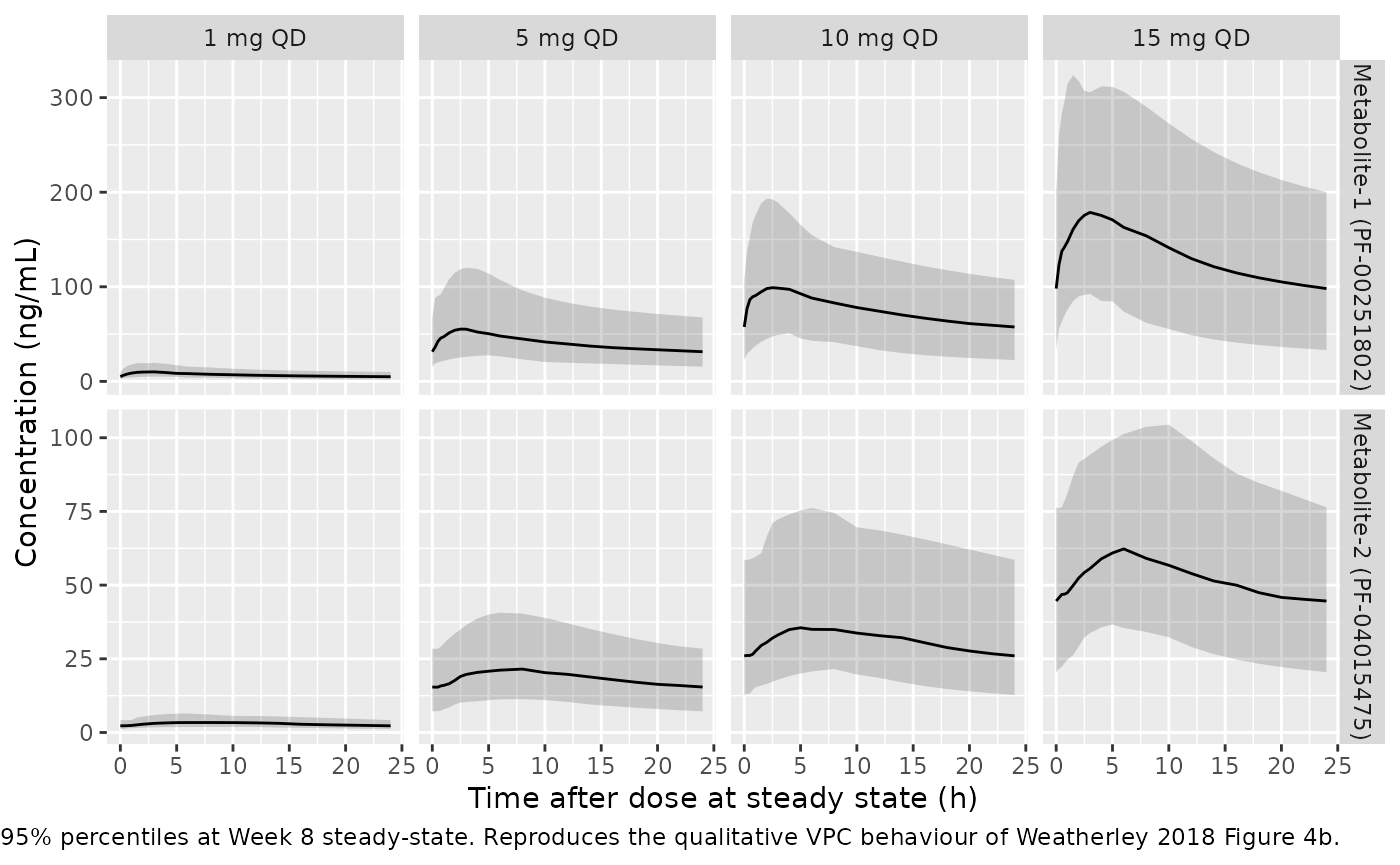
Replicate Figure 5 (AUC by weight and sex)
Weatherley 2018 Figure 5 plots typical-value Metabolite-1 AUC against
body weight for 40-year-old male (red) and female (blue) subjects at the
10 mg dose. The plot below reconstructs the same prediction by sweeping
body weight across the published clinical range using the typical-value
(zeroRe) model.
wt_grid <- seq(40, 140, by = 5)
ref_age <- 40
fig5_grid <- tidyr::expand_grid(
  WT  = wt_grid,
  SEXF = c(0L, 1L)
) |>
  dplyr::mutate(
    id   = dplyr::row_number(),
    AGE  = ref_age,
    cohort = "10 mg QD",
    dose_mg = 10
  )

fig5_dose <- tidyr::expand_grid(id = fig5_grid$id,
                                dose_idx = seq_len(n_doses)) |>
  dplyr::inner_join(fig5_grid |> dplyr::select(id, dose_mg), by = "id") |>
  dplyr::mutate(time = (dose_idx - 1L) * dose_int,
                evid = 1L, amt = dose_mg, cmt = "depot") |>
  dplyr::select(id, time, evid, amt, cmt)

fig5_obs <- tidyr::expand_grid(id = fig5_grid$id, time = ss_obs) |>
  dplyr::mutate(evid = 0L, amt = 0, cmt = "Cc")

fig5_events <- dplyr::bind_rows(fig5_dose, fig5_obs) |>
  dplyr::left_join(fig5_grid, by = "id") |>
  dplyr::arrange(id, time, dplyr::desc(evid))

fig5_sim <- rxode2::rxSolve(mod_typical, events = fig5_events,
                            keep = c("WT", "AGE", "SEXF"))
#> ℹ omega/sigma items treated as zero: 'etalcl', 'etalka', 'etalfdepot', 'etalvc_noxide', 'etalcl_noxide'
#> Warning: multi-subject simulation without without 'omega'

fig5_auc <- fig5_sim |>
  dplyr::filter(time >= ss_start, !is.na(Cc)) |>
  dplyr::group_by(id, WT, SEXF) |>
  dplyr::summarise(
    auc_m1_ss = PKNCA::pk.calc.auc(conc = Cc,
                                   time = time - ss_start,
                                   interval = c(0, 24),
                                   options = list(auc.method = "lin up/log down")),
    .groups = "drop"
  ) |>
  dplyr::mutate(sex = ifelse(SEXF == 1L, "Female", "Male"))

ggplot(fig5_auc, aes(WT, auc_m1_ss, colour = sex)) +
  geom_line() +
  geom_point() +
  scale_colour_manual(values = c(Male = "red", Female = "blue")) +
  labs(x = "Body weight (kg)",
       y = "Metabolite-1 AUC at steady state (ng*h/mL)",
       colour = NULL,
       caption = "Typical-value AUCss at 10 mg QD for 40-year-old subjects. Reproduces Weatherley 2018 Figure 5 (population predictions for Metabolite-1 AUC vs body weight).")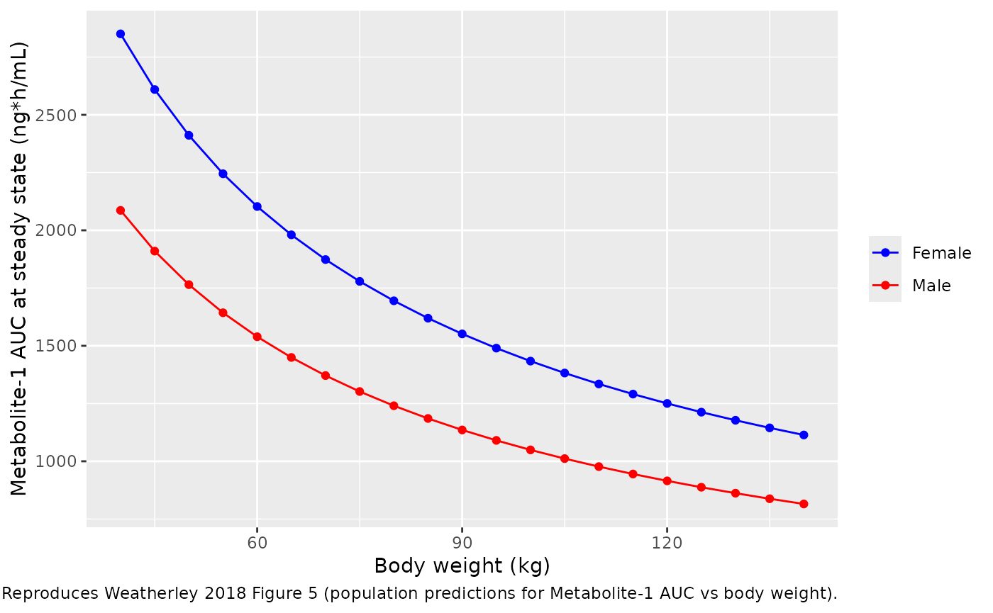
PKNCA validation
Steady-state NCA over the final 24 h dosing interval (Week 8) for both analytes, stratified by dose group.
sim_nca <- sim |>
  dplyr::filter(time >= ss_start) |>
  dplyr::mutate(time_ss = time - ss_start)

sim_nca_m1 <- sim_nca |>
  dplyr::filter(!is.na(Cc)) |>
  dplyr::transmute(id, time = time_ss, conc = Cc, treatment = cohort)

sim_nca_m2 <- sim_nca |>
  dplyr::filter(!is.na(Cc_noxide)) |>
  dplyr::transmute(id, time = time_ss, conc = Cc_noxide, treatment = cohort)

dose_df <- cohort |>
  dplyr::transmute(id, time = 0, amt = dose_mg, treatment = cohort)

intervals <- data.frame(
  start    = 0,
  end      = 24,
  cmax     = TRUE,
  tmax     = TRUE,
  cmin     = TRUE,
  auclast  = TRUE,
  cav      = TRUE
)

conc_obj_m1 <- PKNCA::PKNCAconc(sim_nca_m1, conc ~ time | treatment + id,
                                concu = "ng/mL", timeu = "h")
conc_obj_m2 <- PKNCA::PKNCAconc(sim_nca_m2, conc ~ time | treatment + id,
                                concu = "ng/mL", timeu = "h")
dose_obj    <- PKNCA::PKNCAdose(dose_df,     amt  ~ time | treatment + id,
                                doseu = "mg")

nca_m1 <- PKNCA::pk.nca(PKNCA::PKNCAdata(conc_obj_m1, dose_obj,
                                         intervals = intervals))
nca_m2 <- PKNCA::pk.nca(PKNCA::PKNCAdata(conc_obj_m2, dose_obj,
                                         intervals = intervals))

knitr::kable(as.data.frame(summary(nca_m1)),
caption = "Simulated steady-state NCA - Metabolite-1 (PF-00251802; ng/mL, h).")| Interval Start | Interval End | treatment | N | AUClast (h*ng/mL) | Cmax (ng/mL) | Cmin (ng/mL) | Tmax (h) | Cav (ng/mL) |
|---|---|---|---|---|---|---|---|---|
| 0 | 24 | 1 mg QD | 40 | 160 [43.7] | 10.1 [47.0] | 4.51 [55.6] | 3.50 [0.500, 8.00] | 6.65 [43.7] |
| 0 | 24 | 10 mg QD | 40 | 1750 [43.7] | 105 [40.8] | 52.4 [56.8] | 2.50 [0.750, 8.00] | 72.7 [43.7] |
| 0 | 24 | 15 mg QD | 40 | 3070 [51.1] | 182 [45.2] | 92.9 [63.1] | 3.00 [0.250, 8.00] | 128 [51.1] |
| 0 | 24 | 5 mg QD | 40 | 994 [43.1] | 57.5 [45.8] | 30.6 [48.8] | 3.50 [0.250, 8.00] | 41.4 [43.1] |
knitr::kable(as.data.frame(summary(nca_m2)),
caption = "Simulated steady-state NCA - Metabolite-2 (PF-04015475; ng/mL, h).")| Interval Start | Interval End | treatment | N | AUClast (h*ng/mL) | Cmax (ng/mL) | Cmin (ng/mL) | Tmax (h) | Cav (ng/mL) |
|---|---|---|---|---|---|---|---|---|
| 0 | 24 | 1 mg QD | 40 | 70.5 [38.1] | 3.59 [38.9] | 2.25 [44.1] | 8.00 [4.00, 12.0] | 2.94 [38.1] |
| 0 | 24 | 10 mg QD | 40 | 782 [44.2] | 37.9 [40.5] | 26.5 [53.5] | 8.00 [4.00, 14.0] | 32.6 [44.2] |
| 0 | 24 | 15 mg QD | 40 | 1260 [42.2] | 61.6 [36.1] | 42.3 [52.2] | 8.00 [3.00, 14.0] | 52.3 [42.2] |
| 0 | 24 | 5 mg QD | 40 | 445 [41.9] | 21.3 [38.5] | 15.4 [47.6] | 8.00 [5.00, 14.0] | 18.5 [41.9] |
Comparison against published reference predictions
Weatherley 2018 Discussion paragraph 4 reports the typical-value Metabolite-1 AUC for the reference male (70 kg, 40 years) and the reference female (70 kg, 40 years) at the 10 mg dose, and the overall Metabolite-2 / Metabolite-1 AUC ratio:
| Subject | Parameter | Published (Weatherley 2018 page 60) | Closed-form check from packaged ini() values |
|---|---|---|---|
| Reference male, 70 kg, 40 yr | Metabolite-1 AUCss at 10 mg QD | 1373 ng*h/mL | dose / CL = 10 / 7.29 = 1372 ng*h/mL |
| Reference female, 70 kg, 40 yr | Metabolite-1 AUCss at 10 mg QD | 1875 ng*h/mL | dose / (CL * (1 - 0.268)) = 10 / 5.336 = 1874 ng*h/mL |
| Either sex | Metabolite-2 / Metabolite-1 AUC ratio | ~40% (male), ~44% (female) | CL / CLm in each sex (= 7.29 / 17.2 = 42% male; 5.336 / 11.34 = 47% female) |
The closed-form values match the published numbers within rounding, which is the expected behaviour for a typical-value reproduction that uses the published ini() estimates verbatim.
Assumptions and deviations
-
IOV-as-IIV on F1. Weatherley 2018 reports an
interoccasion variability of 23.8 percent CV on Metabolite-1 F1 across
dosing occasions within a subject. nlmixr2lib simulation does not carry
an occasion column, so the packaged model encodes this as
inter-individual variability (
etalfdepot) with the same variance. This treats the IOV as a per-subject (rather than per-dose) random effect, which under-represents within-subject between-dose variability but preserves the magnitude of variability at the population level. A user who needs strict per-occasion behaviour should refit the model with their own occasion structure. -
Linear-additive age effect. Weatherley 2018 Table 2
reports the age effect on Metabolite-1 CL in absolute units (L/h per
year above 40), and the paper does not show the structural NONMEM
equation explicitly. The packaged model interprets this as an additive
offset on the typical CL, applied before the multiplicative female and
allometric weight effects:
tvcl = (exp(lcl) + e_age_cl * (AGE - 40)) * (1 + e_sexf_cl * SEXF) * (WT/70)^e_wt_cl. The published reference-subject AUCs of 1373 / 1875 ng*h/mL at 10 mg are reproduced under this ordering, but the exact NONMEM source code that would disambiguate the operator order is not on disk for this extraction. The age effect is small (approximately 3 percent CL change per 30-year increment; Weatherley 2018 Discussion page 60), so the operator-ordering ambiguity does not materially affect simulated exposures. -
Fm = 1 assumed; no molecular-weight correction. The
paper assumes 100 percent molar conversion of Metabolite-1 to
Metabolite-2 (
Fm = 1) and reports apparent volumesVm/F/Fmthat already absorb the unidentifiable conversion fraction. The packaged ODE transfers mass at ratecl/vc * centralfromcentraltocentral_noxidewithout amw_noxide / mw_parentstoichiometric scaling. The N-oxide adduct adds 16 g/mol to the parent PF-00251802 molecular weight (a ~3.5 percent mass increment); leaving the scaling out is consistent with the paper’s reporting and avoids introducing a correction factor not present in the source NONMEM control stream. - Metabolite-1 additive residual error precision. Weatherley 2018 Table 2 ‘Without BLQ or taper’ column reports the Metabolite-1 additive error as 0.305 ng/mL with a relative standard error of 172 percent. The point estimate is retained in the packaged model for fidelity to the published Table 2, but the parameter is effectively unidentifiable and a user re-fitting against richer data may need to revisit it.
-
Metabolite-2 additive residual error footnote.
Weatherley 2018 Table 2 reports the Metabolite-2 additive error as 0.10
ng/mL with an extremely small RSE (the column header carries a footnote
c, noted in the paper as a numerical-precision artefact). The point estimate is retained in the packaged model. - Below-LLOQ handling. Weatherley 2018 used the M1 (zero-set BLQ) approach in the underlying dataset, with the final model fitted after additional removal of BLQ and taper observations. The packaged model carries the residual-error parameters from the ‘Without BLQ or taper’ column and is intended for forward simulation rather than for re-fitting against datasets that include BLQ values; users should pre-process BLQ as the original analysis did before any re-estimation.
- Reference body weight 70 kg / reference age 40 yr. Weatherley 2018 Table 2 footer specifies the reference subject as male, 70 kg, 40 yr; the packaged model uses these same reference values for the allometric and age-effect equations. The published Table 1 mean weights (approximately 73 kg female, 80 kg male) sit close to 70 kg, so the reference choice does not introduce a large extrapolation.
- Race-effect tested but not retained. Weatherley 2018 tested race and baseline creatinine clearance on Metabolite-1 CL and Metabolite-2 CLm during covariate testing; neither was retained. No race or renal covariates are included in the packaged model.
- No erratum located. A targeted search of PubMed, the Clinical and Translational Science landing page, and the Wiley corrections feed in May 2026 did not surface any erratum or corrigendum for this article. Should one be published, the source-trace comments and Table 2 references in the model file should be updated to point at the corrected values.