Atractylodes lancea in advanced intrahepatic cholangiocarcinoma (Saeheng 2024)
Source:vignettes/articles/Saeheng_2024_atractylodesLancea.Rmd
Saeheng_2024_atractylodesLancea.RmdModel and source
Saeheng 2024 fitted the same structural model – one compartment, zero-order absorption without delay, linear clearance – separately to three sampling occasions, and reported the three parameter sets in Tables 1, 2 and 3. The library therefore carries three model files that share this vignette.
| Model | Source table | Occasion |
|---|---|---|
Saeheng_2024_atractylodesLancea_group1day1 |
Table 1 | Group 1, day 1 (first 1,000 mg dose) |
Saeheng_2024_atractylodesLancea_group2day14 |
Table 2 | Group 2, day 14 (end of the 1,000 mg lead-in) |
Saeheng_2024_atractylodesLancea_group2day28 |
Table 3 | Group 2, day 28 (end of the 1,500 mg step) |
- Citation: Saeheng T, Karbwang J, Na-Bangchang K. Population-pharmacokinetic/pharmacodynamic model of atractylodes lancea (Thunb.) DC. administration in patients with advanced-stage intrahepatic cholangiocarcinoma: a dosage prediction. BMC Complement Med Ther. 2024;24(1):384. doi:10.1186/s12906-024-04618-8.
- Description (Group 1, day 1): One-compartment population PK model with zero-order absorption (no lag) and linear clearance for total Atractylodes lancea (Thunb.) DC. bioactivity in patients with advanced-stage intrahepatic cholangiocarcinoma (Saeheng 2024, Table 1). This file holds the Group 1 day-1 fit: the first once-daily 1,000 mg dose of the capsule formulation of standardized AL extract (CMC-AL). Saeheng 2024 reported three separate fits of the same structural model to three different occasions – Group 1 day 1, Group 2 day 14 and Group 2 day 28 – carried here as three model files sharing one vignette; see also modellib(‘Saeheng_2024_atractylodesLancea_group2day14’) and modellib(‘Saeheng_2024_atractylodesLancea_group2day28’). Volume and clearance are apparent (V/F, CL/F): CMC-AL is dosed orally and no bioavailability term was estimated. The analyte is total AL bioactivity, a bioassay-derived aggregate of the extract’s active constituents, not a single molecular entity. None of the screened covariates (sex, age, weight, height) improved the model. Between-subject variability is lognormal on Tk0, V/F and CL/F; residual error is combined additive plus proportional.
- Article: https://doi.org/10.1186/s12906-024-04618-8
- Trial registration: TCTR20210129007 (https://www.thaiclinicaltrials.org)
The drug is CMC-AL, a capsule formulation of a standardized extract
of Atractylodes lancea (Thunb.) DC. The analyte is
total AL bioactivity, a bioassay-derived aggregate of
the extract’s active constituents rather than a single molecular entity,
so V/F and CL/F are apparent parameters of
that aggregate. Saeheng 2024 also developed a pop-PK model for
atractylodin (a single active constituent) but reported no parameters
for it and did not use it for dose prediction, so it is not carried
here.
Population
Data come from the Group 1 and Group 2 arms of a single-centre, open-label, randomized, controlled phase 2A trial in patients with advanced-stage intrahepatic cholangiocarcinoma (iCCA) at Sakhon Na-Kon Hospital, Thailand (TCTR20210129007). Group 1 (n = 15) received 1,000 mg CMC-AL once daily (9 capsules) for 90 days. Group 2 (n = 16) received an escalating regimen: 1,000 mg once daily for 14 days, then 1,500 mg once daily for 14 days, then 2,000 mg once daily for 62 days. Group 3 (n = 16) was a standard-supportive-care control arm and contributed no PK. All arms received standard supportive care.
Plasma was sampled at 0, 0.25, 0.5, 1, 1.5, 2, 2.5, 3, 4, 5, 6 and 8
h post-dose: on day 1 for Group 1, and on days 14 and 28 for Group 2.
None of the screened covariates (sex, age, weight, height) improved the
model, so the final model has no covariate terms; the screen is recorded
in each model file’s covariatesDataExcluded metadata.
Saeheng 2024 does not tabulate baseline demographics
(age, weight, sex, height) for the PK cohort – those are reported in the
parent phase 2A trial publication (its reference [8]). The
population metadata therefore carries the design facts
only.
readModelDb("Saeheng_2024_atractylodesLancea_group1day1")()$population$notes
#> [1] "Group 1 arm of a single-centre, open-label, randomized, controlled phase 2A trial (TCTR20210129007). Fifteen patients were randomized to Group 1 (Saeheng 2024 Results). Plasma sampling on day 1 at 0, 0.25, 0.5, 1, 1.5, 2, 2.5, 3, 4, 5, 6 and 8 h post-dose (Saeheng 2024 Methods, 'Pharmacokinetic study'). Baseline demographics (age, weight, sex, height) are not tabulated in this paper; they are reported in the parent phase 2A trial publication (reference [8]). Fitted in MonolixSuite 2023R1 by SAEM."
Source trace
Every ini() entry carries an in-file comment naming its
source cell in Saeheng 2024. They are collected here for review.
| Equation / parameter | Group 1 day 1 (Table 1) | Group 2 day 14 (Table 2) | Group 2 day 28 (Table 3) |
|---|---|---|---|
ld1 = log(Tk0), zero-order absorption duration (h) |
0.85 (RSE 17.3%) | 1.11 (RSE 11.2%) | 0.95 (RSE 9.10%) |
lvc = log(V/F) (L) |
42.82 (RSE 11.3%) | 32.57 (RSE 8.89%) | 32 (RSE 7.85%) |
lcl = log(CL/F) (L/h) |
20.9 (RSE 16.1%) | 17.2 (RSE 11.8%) | 16.13 (RSE 10.7%) |
etald1 variance |
0.51^2 (Omega_Tk0) | 0.35^2 (Omega_Tk0) | 0.28^2 (Omega_Tk0) |
etalvc variance |
log(1 + 0.3082^2), from the printed %CV – see Errata | log(1 + 0.273^2), from the printed %CV – see Errata | 0.25^2 (Omega_V) |
etalcl variance |
0.54^2 (Omega_Cl) | 0.44^2 (Omega_Cl) | 0.38^2 (Omega_Cl) |
addSd (mg/L) |
a = 0.36 (RSE 28.4%) | a = 1.39 (RSE 24.0%) | a = 2.21 (RSE 19.2%) |
propSd (fraction) |
b = 0.32 (RSE 11.8%) | b = 0.17 (RSE 19.3%) | b = 0.084 (RSE 29.6%) |
d/dt(central) <- -kel * central,
dur(central) <- d1
|
Results: “One compartmental model with zero-order absorption (without delay) and linear clearance best characterized the pop-PK properties of total bioactivity of AL” | same | same |
Cc <- central / vc |
Methods, “Criteria for optimal dosage regimens” (Cmax cut-offs quoted in mg/L) | same | same |
| Cmax cut-offs 32.39 / 21.42 mg/L | Methods, “Criteria for optimal dosage regimens” | – | – |
| Published MC outcome percentages | Results, “Tumor progression” and “Deaths” | – | – |
Virtual cohort
Original observed data are not publicly available. Each occasion is reproduced with a virtual cohort of 200 subjects dosed on the schedule that applied to that occasion, and sampled over the 0-8 h window the protocol used. The model has no covariates, so no covariate distribution has to be assumed.
set.seed(20240384)

N_PER_ARM <- 200L

# Protocol sampling times (Methods, "Pharmacokinetic study").
protocol_times <- c(0, 0.25, 0.5, 1, 1.5, 2, 2.5, 3, 4, 5, 6, 8)

# Dense grid for the closed-form NCA gate; the union keeps the protocol times
# available for the population NCA. The typical Tk0 of each occasion (0.85,
# 1.11, 0.95 h) is added so PKNCA can land exactly on the analytic Tmax.
obs_times <- sort(unique(c(seq(0, 8, by = 0.05), protocol_times, 0.85, 1.11, 0.95)))

# Build one occasion: `dose_times` / `dose_amts` give the full dosing history in
# absolute hours; `occasion_time` is the absolute time of the dose being
# sampled. `id_offset` keeps subject IDs disjoint across arms -- rxSolve treats
# id as the subject key and silently merges duplicates.
make_occasion <- function(occasion, n, dose_times, dose_amts, occasion_time,
                          id_offset = 0L) {
  ids <- id_offset + seq_len(n)
  doses <- tidyr::expand_grid(id = ids, k = seq_along(dose_times)) |>
    dplyr::mutate(
      time = dose_times[k],
      amt  = dose_amts[k],
      evid = 1L,
      rate = -2      # use the modelled dur(central) for the zero-order input
    ) |>
    dplyr::select(-k)
  obs <- tidyr::expand_grid(id = ids, time = occasion_time + obs_times) |>
    dplyr::mutate(amt = NA_real_, evid = 0L, rate = 0)
  dplyr::bind_rows(doses, obs) |>
    dplyr::mutate(
      cmt      = "central",       # the ODE state, never the observable "Cc"
      occasion = occasion,
      occasion_time = occasion_time,
      dose_mg  = dose_amts[length(dose_amts)]
    ) |>
    dplyr::arrange(id, time, dplyr::desc(evid))
}

# Group 1: single 1,000 mg dose, sampled on day 1.
ev_g1d1 <- make_occasion(
  "Group 1, day 1 (1,000 mg)", N_PER_ARM,
  dose_times = 0, dose_amts = 1000, occasion_time = 0, id_offset = 0L
)

# Group 2 day 14: 14 daily 1,000 mg doses; day-14 dose is at t = 13 * 24 h.
g2_lead_times <- seq(0, by = 24, length.out = 14)
ev_g2d14 <- make_occasion(
  "Group 2, day 14 (1,000 mg)", N_PER_ARM,
  dose_times = g2_lead_times, dose_amts = rep(1000, 14),
  occasion_time = 13 * 24, id_offset = 200L
)

# Group 2 day 28: the 1,000 mg lead-in followed by 14 daily 1,500 mg doses;
# day-28 dose is at t = 27 * 24 h.
g2_step_times <- seq(14 * 24, by = 24, length.out = 14)
ev_g2d28 <- make_occasion(
  "Group 2, day 28 (1,500 mg)", N_PER_ARM,
  dose_times = c(g2_lead_times, g2_step_times),
  dose_amts  = c(rep(1000, 14), rep(1500, 14)),
  occasion_time = 27 * 24, id_offset = 400L
)

events <- dplyr::bind_rows(ev_g1d1, ev_g2d14, ev_g2d28)
stopifnot(!anyDuplicated(unique(events[, c("id", "time", "evid")])))
Simulation
Each occasion is solved with its own parameter set, then the three results are stacked. A separate typical-value (deterministic) solve backs the closed-form NCA gate below.
occasion_model <- c(
  "Group 1, day 1 (1,000 mg)"  = "Saeheng_2024_atractylodesLancea_group1day1",
  "Group 2, day 14 (1,000 mg)" = "Saeheng_2024_atractylodesLancea_group2day14",
  "Group 2, day 28 (1,500 mg)" = "Saeheng_2024_atractylodesLancea_group2day28"
)

solve_occasion <- function(occ, typical) {
  # Read a fresh copy per solve: zeroRe() mutates the model object it is given.
  mod <- readModelDb(occasion_model[[occ]])
  ev  <- events |> dplyr::filter(occasion == occ)
  if (typical) {
    # One representative subject: with the etas zeroed every subject is
    # identical, and a single profile is what the closed-form gate needs.
    ev <- ev |> dplyr::filter(id == min(id))
    # omega = NA is required in addition to zeroRe(): rxode2 otherwise re-samples
    # etas once a stochastic solve has run in the same session.
    out <- rxode2::rxSolve(rxode2::zeroRe(mod), events = ev, omega = NA,
                           keep = c("occasion", "occasion_time", "dose_mg"))
  } else {
    out <- rxode2::rxSolve(mod, events = ev,
                           keep = c("occasion", "occasion_time", "dose_mg"))
  }
  out <- as.data.frame(out)
  # rxSolve drops the id column for a single-subject solve; restore it so the
  # downstream PKNCA grouping works for both branches.
  if (!"id" %in% names(out)) out$id <- ev$id[[1]]
  out
}

sim_pop <- dplyr::bind_rows(lapply(names(occasion_model), solve_occasion,
                                   typical = FALSE)) |>
  dplyr::mutate(tad = time - occasion_time)
#> ℹ parameter labels from comments will be replaced by 'label()'
#> ℹ parameter labels from comments will be replaced by 'label()'
#> ℹ parameter labels from comments will be replaced by 'label()'

sim_typ <- dplyr::bind_rows(lapply(names(occasion_model), solve_occasion,
                                   typical = TRUE)) |>
  dplyr::mutate(tad = time - occasion_time)
#> ℹ parameter labels from comments will be replaced by 'label()'
#> ℹ parameter labels from comments will be replaced by 'label()'
#> ℹ parameter labels from comments will be replaced by 'label()'
Replicate published figures
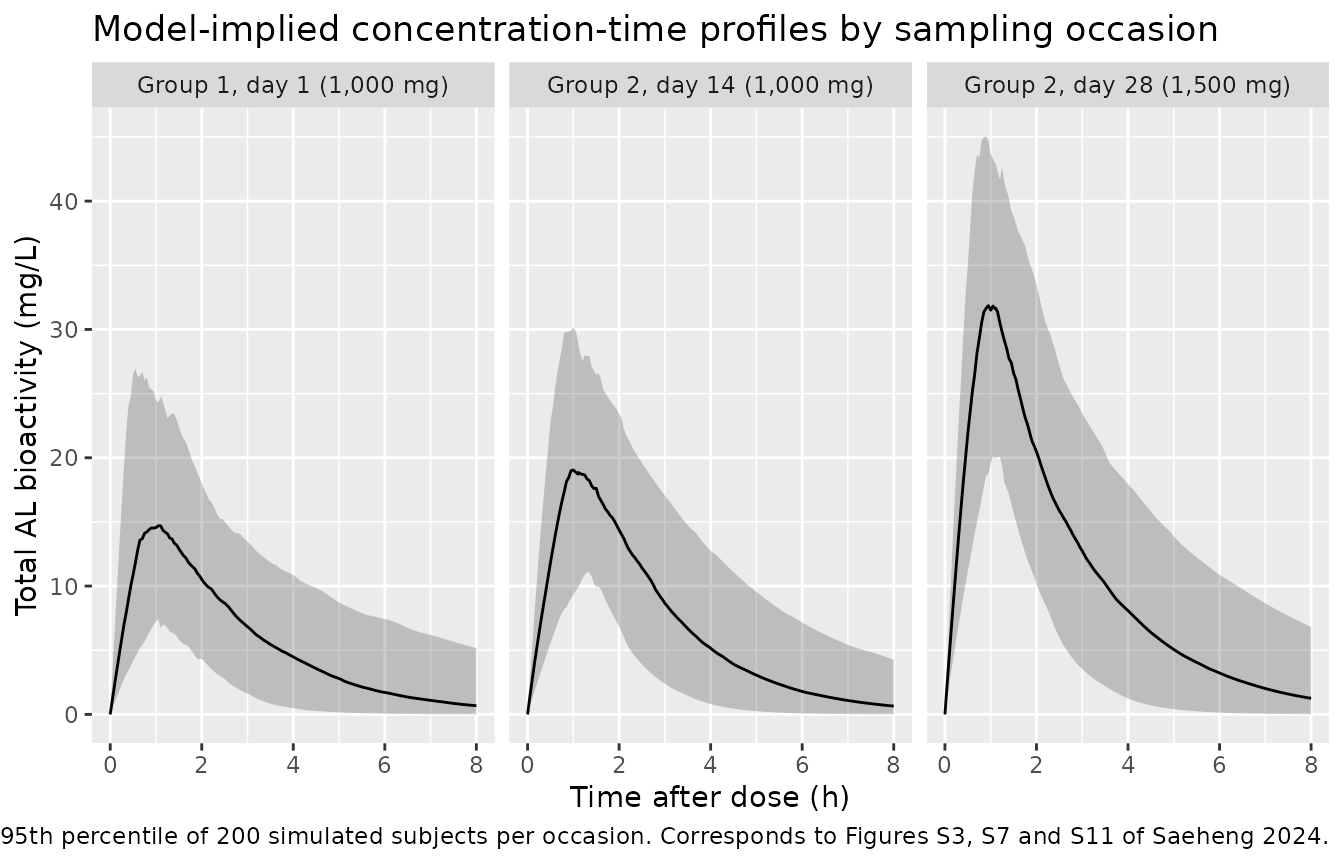
Saeheng 2024 shows the per-occasion concentration-time profiles and their visual predictive checks in Supplementary Figures S1-S12 (Additional File 1), which are not reproduced numerically in the article text. The panels below are the model-implied equivalents of Figures S3, S7 and S11 (the VPCs for Group 1 day 1, Group 2 day 14 and Group 2 day 28).
sim_pop |>
  dplyr::filter(!is.na(Cc)) |>
  dplyr::group_by(occasion, tad) |>
  dplyr::summarise(
    Q05 = quantile(Cc, 0.05),
    Q50 = quantile(Cc, 0.50),
    Q95 = quantile(Cc, 0.95),
    .groups = "drop"
  ) |>
  ggplot(aes(tad, Q50)) +
  geom_ribbon(aes(ymin = Q05, ymax = Q95), alpha = 0.25) +
  geom_line() +
  facet_wrap(~occasion) +
  labs(
    x = "Time after dose (h)", y = "Total AL bioactivity (mg/L)",
    title = "Model-implied concentration-time profiles by sampling occasion",
    caption = paste("Median and 5th-95th percentile of 200 simulated subjects per occasion.",
                    "Corresponds to Figures S3, S7 and S11 of Saeheng 2024.")
  )
PKNCA validation
Closed-form gate on the typical-value profiles
For a one-compartment model with a zero-order input of duration
d1 and no accumulation, NCA parameters have exact closed
forms: Tmax = d1,
Cmax = (D / (d1 * CL)) * (1 - exp(-kel * d1)),
AUC(0-inf) = D / CL, and t1/2 = log(2) / kel.
Terminal half-lives here are 1.3-1.4 h against a 24 h dosing interval,
so the accumulation contribution to Cmax is below 1e-5 of the peak and
the single-dose forms apply on days 14 and 28 as well; the accumulation
ratio is checked numerically below. PKNCA run on the typical-value
profile must reproduce these values – this is a strict check of the
packaged implementation, not a tuned comparison.
# Accumulation ratio actually observed in the simulated typical profiles: the
# pre-dose (trough) concentration relative to the same occasion's peak.
sim_typ |>
  dplyr::group_by(occasion) |>
  dplyr::summarise(
    `Cmax (mg/L)`        = max(Cc),
    `Pre-dose Cc (mg/L)` = Cc[tad == 0],
    `Trough / Cmax`      = Cc[tad == 0] / max(Cc),
    .groups = "drop"
  ) |>
  knitr::kable(digits = c(0, 3, 8, 8),
caption = "Accumulation is negligible: the pre-dose concentration on days 14 and 28 is a vanishing fraction of the peak.")| occasion | Cmax (mg/L) | Pre-dose Cc (mg/L) | Trough / Cmax |
|---|---|---|---|
| Group 1, day 1 (1,000 mg) | 19.115 | 0.00000000 | 0.00e+00 |
| Group 2, day 14 (1,000 mg) | 23.232 | 0.00013071 | 5.63e-06 |
| Group 2, day 28 (1,500 mg) | 37.248 | 0.00033511 | 9.00e-06 |
nca_frame <- function(dat) {
  out <- dat |>
    dplyr::filter(!is.na(Cc)) |>
    dplyr::select(id, tad, Cc, occasion, dose_mg)
  # Guarantee a tad = 0 row per (id, occasion); pre-dose Cc = 0 is correct for
  # an extravascular first dose and negligible on days 14 / 28.
  dplyr::bind_rows(
    out,
    out |> dplyr::distinct(id, occasion, dose_mg) |>
      dplyr::mutate(tad = 0, Cc = 0)
  ) |>
    dplyr::distinct(id, occasion, tad, .keep_all = TRUE) |>
    dplyr::arrange(occasion, id, tad)
}

nca_intervals <- data.frame(
  start = 0, end = Inf,
  cmax = TRUE, tmax = TRUE, aucinf.obs = TRUE, half.life = TRUE
)

run_nca <- function(conc_df) {
  dose_df <- conc_df |>
    dplyr::distinct(id, occasion, dose_mg) |>
    dplyr::mutate(time = 0, amt = dose_mg)
  PKNCA::pk.nca(PKNCA::PKNCAdata(
    PKNCA::PKNCAconc(conc_df, Cc ~ tad | occasion + id),
    PKNCA::PKNCAdose(dose_df, amt ~ time | occasion + id),
    intervals = nca_intervals
  ))
}

nca_typ <- run_nca(nca_frame(sim_typ))
closed_form <- tibble::tribble(
  ~occasion,                     ~d1,   ~vc,    ~cl,    ~dose,
  "Group 1, day 1 (1,000 mg)",   0.85,  42.82,  20.90,  1000,
  "Group 2, day 14 (1,000 mg)",  1.11,  32.57,  17.20,  1000,
  "Group 2, day 28 (1,500 mg)",  0.95,  32.00,  16.13,  1500
) |>
  dplyr::mutate(
    kel        = cl / vc,
    cmax       = (dose / (d1 * cl)) * (1 - exp(-kel * d1)),
    tmax       = d1,
    aucinf.obs = dose / cl,
    half.life  = log(2) / kel
  ) |>
  dplyr::select(occasion, cmax, tmax, aucinf.obs, half.life)

nlmixr2lib::ncaComparisonTable(
  simulated = nca_typ,
  reference = closed_form,
  by        = "occasion",
  units     = c(cmax = "mg/L", tmax = "h", aucinf.obs = "mg*h/L", half.life = "h"),
  tolerance_pct = 20
) |>
  knitr::kable(
    digits  = 3,
    caption = "Typical-value PKNCA output vs. the exact closed-form solution of the packaged model. * marks a >20% difference."
)| NCA parameter | occasion | Reference | Simulated | % diff |
|---|---|---|---|---|
| Cmax (mg/L) | Group 1, day 1 (1,000 mg) | 19.1 | 19.1 | -0.0% |
| Cmax (mg/L) | Group 2, day 14 (1,000 mg) | 23.2 | 23.2 | +0.0% |
| Cmax (mg/L) | Group 2, day 28 (1,500 mg) | 37.2 | 37.2 | +0.0% |
| Tmax (h) | Group 1, day 1 (1,000 mg) | 0.85 | 0.85 | +0.0% |
| Tmax (h) | Group 2, day 14 (1,000 mg) | 1.11 | 1.11 | +0.0% |
| Tmax (h) | Group 2, day 28 (1,500 mg) | 0.95 | 0.95 | +0.0% |
| AUC0-∞ (obs) (mg*h/L) | Group 1, day 1 (1,000 mg) | 47.8 | 47.8 | -0.0% |
| AUC0-∞ (obs) (mg*h/L) | Group 2, day 14 (1,000 mg) | 58.1 | 58.1 | -0.0% |
| AUC0-∞ (obs) (mg*h/L) | Group 2, day 28 (1,500 mg) | 93 | 93 | -0.0% |
| t½ (h) | Group 1, day 1 (1,000 mg) | 1.42 | 1.42 | +0.0% |
| t½ (h) | Group 2, day 14 (1,000 mg) | 1.31 | 1.31 | +0.0% |
| t½ (h) | Group 2, day 28 (1,500 mg) | 1.38 | 1.38 | +0.0% |
Population NCA on the protocol sampling times
Restricting the simulated cohort to the 12 protocol sampling times gives the NCA a study-realistic design. Saeheng 2024 reports no NCA table, so these values are descriptive rather than a comparison target; note that the sparse grid puts Tmax on the nearest protocol time (1 h) rather than on the true Tk0.
nca_pop <- sim_pop |>
  dplyr::filter(tad %in% protocol_times) |>
  nca_frame() |>
  run_nca()

as.data.frame(nca_pop) |>
  dplyr::filter(PPTESTCD %in% c("cmax", "tmax", "aucinf.obs", "half.life")) |>
  dplyr::group_by(occasion, PPTESTCD) |>
  dplyr::summarise(
    Median = median(PPORRES, na.rm = TRUE),
    `5th`  = quantile(PPORRES, 0.05, na.rm = TRUE),
    `95th` = quantile(PPORRES, 0.95, na.rm = TRUE),
    .groups = "drop"
  ) |>
  tidyr::pivot_longer(c(Median, `5th`, `95th`)) |>
  tidyr::pivot_wider(names_from = PPTESTCD, values_from = value) |>
  dplyr::rename(
    "Occasion"          = occasion,
    "Statistic"         = name,
    "Cmax (mg/L)"       = cmax,
    "Tmax (h)"          = tmax,
    "AUC0-inf (mg*h/L)" = aucinf.obs,
    "t1/2 (h)"          = half.life
  ) |>
  knitr::kable(digits = 2,
caption = "Simulated population NCA on the protocol sampling grid (200 subjects per occasion).")| Occasion | Statistic | AUC0-inf (mg*h/L) | Cmax (mg/L) | t1/2 (h) | Tmax (h) |
|---|---|---|---|---|---|
| Group 1, day 1 (1,000 mg) | Median | 47.54 | 16.17 | 1.43 | 1.0 |
| Group 1, day 1 (1,000 mg) | 5th | 20.70 | 9.50 | 0.59 | 0.5 |
| Group 1, day 1 (1,000 mg) | 95th | 111.74 | 28.49 | 4.08 | 2.0 |
| Group 2, day 14 (1,000 mg) | Median | 58.27 | 20.19 | 1.36 | 1.0 |
| Group 2, day 14 (1,000 mg) | 5th | 24.74 | 13.99 | 0.55 | 0.5 |
| Group 2, day 14 (1,000 mg) | 95th | 124.69 | 29.14 | 3.15 | 2.0 |
| Group 2, day 28 (1,500 mg) | Median | 94.51 | 33.97 | 1.50 | 1.0 |
| Group 2, day 28 (1,500 mg) | 5th | 56.52 | 23.25 | 0.78 | 0.5 |
| Group 2, day 28 (1,500 mg) | 95th | 164.81 | 47.09 | 2.59 | 1.5 |
Reproducing the published dose-selection simulations
This is the paper’s principal quantitative result. Saeheng 2024 ran Monte-Carlo simulations of once-daily regimens of 1,000-3,000 mg and classified a simulated patient using the total-AL-bioactivity Cmax cut-offs quoted in Methods, “Criteria for optimal dosage regimens”: Cmax >= 32.39 mg/L for inhibition of tumour progression, and Cmax >= 21.42 mg/L for prevention of death. The published proportions are in Results, “Tumor progression” and “Deaths” (100% adherence, 3-month course).
The paper does not say which of its three parameter sets drove the simulations. Reproducing all three shows that only the Group 1, day 1 fit lands in the published range, so that is the set used here.
mc_doses <- c(1000, 1500, 2000, 2500, 3000)
MC_PER_ARM <- 200L

# Three daily doses, Cmax taken over the final interval. With t1/2 ~ 1.4 h
# against a 24 h interval this is indistinguishable from the 3-month steady
# state used in the paper (see the accumulation check above).
mc_events <- dplyr::bind_rows(lapply(seq_along(mc_doses), function(k) {
  D   <- mc_doses[k]
  ids <- 1000L + (k - 1L) * MC_PER_ARM + seq_len(MC_PER_ARM)
  doses <- tidyr::expand_grid(id = ids, time = c(0, 24, 48)) |>
    dplyr::mutate(amt = D, evid = 1L, rate = -2)
  obs <- tidyr::expand_grid(id = ids,
                            time = 48 + sort(unique(c(seq(0, 8, by = 0.05),
                                                      protocol_times)))) |>
    dplyr::mutate(amt = NA_real_, evid = 0L, rate = 0)
  dplyr::bind_rows(doses, obs) |>
    dplyr::mutate(cmt = "central", dose_mg = D,
                  regimen = paste0(format(D, big.mark = ","), " mg once daily")) |>
    dplyr::arrange(id, time, dplyr::desc(evid))
}))
stopifnot(!anyDuplicated(unique(mc_events[, c("id", "time", "evid")])))
CUT_PROGRESSION <- 32.39   # mg/L, Methods "Criteria for optimal dosage regimens"
CUT_DEATH       <- 21.42   # mg/L, same

# The paper does not say whether its simulated Cmax is the individual's
# predicted peak or a simulated *measured* peak (Simulx simulates observations
# through the residual-error model by default). Both readings are carried:
#   cmax_pred -- max of Cc  (IPRED), the true individual peak;
#   cmax_obs  -- max of sim (residual error included) restricted to the 12
#                protocol sampling times, i.e. a measured Cmax under the
#                study's own sampling design.
mc_outcomes <- function(model_name) {
  s <- as.data.frame(rxode2::rxSolve(readModelDb(model_name), events = mc_events,
                                     keep = c("dose_mg", "regimen")))
  s |>
    dplyr::filter(!is.na(Cc)) |>
    dplyr::mutate(tad = time - 48) |>
    dplyr::group_by(regimen, dose_mg, id) |>
    dplyr::summarise(
      cmax_pred = max(Cc),
      cmax_obs  = max(sim[tad %in% protocol_times]),
      .groups   = "drop"
    ) |>
    dplyr::group_by(regimen, dose_mg) |>
    dplyr::summarise(
      progression_pred = 100 * mean(cmax_pred < CUT_PROGRESSION),
      death_pred       = 100 * mean(cmax_pred < CUT_DEATH),
      progression_obs  = 100 * mean(cmax_obs  < CUT_PROGRESSION),
      death_obs        = 100 * mean(cmax_obs  < CUT_DEATH),
      .groups = "drop"
    ) |>
    dplyr::mutate(model = model_name)
}

set.seed(384)
mc_all <- dplyr::bind_rows(lapply(unname(occasion_model), mc_outcomes))
#> ℹ parameter labels from comments will be replaced by 'label()'
#> ℹ parameter labels from comments will be replaced by 'label()'
#> ℹ parameter labels from comments will be replaced by 'label()'
published <- tibble::tribble(
  ~dose_mg, ~pub_progression, ~pub_death,
  1000,     96,               66,
  1500,     83,               50,
  2000,     55,               29,
  2500,     27,               12,
  3000,     12,                3
)

mc_all |>
  dplyr::filter(model == "Saeheng_2024_atractylodesLancea_group1day1") |>
  dplyr::left_join(published, by = "dose_mg") |>
  dplyr::arrange(dose_mg) |>
  dplyr::select(regimen, pub_progression, progression_pred, progression_obs,
                pub_death, death_pred, death_obs) |>
  dplyr::rename(
    "Regimen"                     = regimen,
    "Progression, published %"    = pub_progression,
    "Progression, pred. Cmax %"   = progression_pred,
    "Progression, obs. Cmax %"    = progression_obs,
    "Mortality, published %"      = pub_death,
    "Mortality, pred. Cmax %"     = death_pred,
    "Mortality, obs. Cmax %"      = death_obs
  ) |>
  knitr::kable(
    digits  = 1,
    caption = paste("Reproduction of Saeheng 2024 Results ('Tumor progression', 'Deaths') using the",
                    "Group 1 day-1 parameter set, 200 virtual patients per dose arm,",
                    "and the published Cmax cut-offs (32.39 and 21.42 mg/L).",
                    "'pred. Cmax' uses the individual predicted peak; 'obs. Cmax' uses a",
                    "residual-error-included peak on the 12 protocol sampling times.")
)| Regimen | Progression, published % | Progression, pred. Cmax % | Progression, obs. Cmax % | Mortality, published % | Mortality, pred. Cmax % | Mortality, obs. Cmax % |
|---|---|---|---|---|---|---|
| 1,000 mg once daily | 96 | 99.0 | 94.0 | 66 | 72.5 | 65.5 |
| 1,500 mg once daily | 83 | 71.5 | 63.5 | 50 | 16.5 | 24.5 |
| 2,000 mg once daily | 55 | 38.0 | 34.0 | 29 | 5.0 | 8.0 |
| 2,500 mg once daily | 27 | 15.0 | 15.0 | 12 | 1.0 | 2.0 |
| 3,000 mg once daily | 12 | 5.0 | 7.5 | 3 | 0.0 | 0.0 |
The packaged model reproduces the direction of the published dose-response and matches the 1,000 mg anchor closely (published 96% progression / 66% mortality; simulated 94% / 66% on the observed-Cmax reading). It does not reproduce the published intermediate-dose proportions: at 1,500-2,500 mg the simulation is 10-35 percentage points more optimistic than published under either reading, and the gap is largest for mortality.
The reason is structural rather than a transcription problem. The published curves are much shallower than a Cmax-threshold rule can be on this model: over a 3-fold dose range (1,000 to 3,000 mg) the published mortality falls only from 66% to 3%, whereas a fixed cut-off applied to a lognormal Cmax distribution with the model’s variability falls far faster, because tripling the dose triples every individual’s Cmax. Matching the published shallowness would require a Cmax distribution far wider than the reported IIV and residual error imply. Nothing has been tuned to close the gap; the discrepancy is reported as found and noted in Assumptions and deviations below.
mc_all |>
  dplyr::left_join(published, by = "dose_mg") |>
  dplyr::mutate(model = sub("^Saeheng_2024_atractylodesLancea_", "", model)) |>
  dplyr::select(dose_mg, model, progression_obs, pub_progression) |>
  tidyr::pivot_wider(names_from = model, values_from = progression_obs) |>
  dplyr::arrange(dose_mg) |>
  dplyr::rename(
    "Dose (mg once daily)"    = dose_mg,
    "Published progression %" = pub_progression
  ) |>
  knitr::kable(
    digits  = 1,
    caption = paste("Tumour-progression percentage by parameter set (observed-Cmax reading).",
                    "All three agree at 1,000 mg; the sets separate at higher doses, where only",
                    "the Group 1 day-1 fit stays near the published values. The day-14 and",
                    "day-28 fits give markedly higher exposure and therefore far less predicted",
                    "progression.")
)| Dose (mg once daily) | Published progression % | group1day1 | group2day14 | group2day28 |
|---|---|---|---|---|
| 1000 | 96 | 94.0 | 91.5 | 95.5 |
| 1500 | 83 | 63.5 | 49.0 | 40.0 |
| 2000 | 55 | 34.0 | 19.0 | 8.5 |
| 2500 | 27 | 15.0 | 2.5 | 0.5 |
| 3000 | 12 | 7.5 | 0.0 | 0.5 |
Assumptions and deviations
-
Omega_Vin Tables 1 and 2 is printed on the wrong scale. Every other random-effect row in the paper is a Monolix log-scale SD, consistent with the printed%CVcolumn viaCV = sqrt(exp(omega^2) - 1). TheOmega_VValue and S.E. cells of Table 1 (13.2, 4.25) and Table 2 (8.89, 2.44) are not: as log-scale SDs they would imply CVs of ~1e40% and ~1e19%, against printed CVs of 30.82% and 27.3%. They are instead SDs ofVon the linear scale (13.2 / 42.82 = 30.83%; 8.89 / 32.57 = 27.29%), and their%RSEcells are self-consistent on that scale too (4.25 / 13.2 = 32.2%; 2.44 / 8.89 = 27.4%). Table 2’s 8.89 is also the number printed asV_pop’s%RSEtwo rows above, consistent with a transcription slip. Table 3’sOmega_V(0.25) follows the log-scale convention like everything else. Because the paper’s Methods state that “the distribution of pharmacokinetic parameters was normal in a logarithmic scale”, the model files use log-scale omegas recovered from the self-consistent%CVcolumn,omega = sqrt(log(1 + CV^2)): 0.3012 for Table 1 and 0.2681 for Table 2. Both readings imply the same practical variability (~31% and ~27% CV onV/F), so the choice is not material. -
Combined residual-error variance form. Saeheng 2024
reports Monolix
aandberror-model parameters but does not state whether thecombined1(sd = a + b*f) orcombined2(sd = sqrt(a^2 + (b*f)^2)) form was used. rxode2’s defaultcombined2form is used, matching the existing library precedent (Chen_2024_febuxostat). At the observed concentrations the two forms differ by up to ~30% in residual SD on day 28, where the additive term is largest; the structural parameters are unaffected. - Which parameter set drove the Monte-Carlo simulations is not stated. Saeheng 2024 refers only to “the final pop-PK (1000 virtual patients) model”. The comparison above shows the Group 1 day-1 fit is the only one of the three close to the published outcome percentages, so it is used for the dose-selection reproduction.
- The published dose-selection percentages are only partly reproducible. The packaged model plus the published Cmax cut-offs matches the 1,000 mg outcomes closely and reproduces the direction of the dose-response, but is 10-35 percentage points more optimistic than published at 1,500-2,500 mg under both the predicted-Cmax and observed-Cmax readings. The published curves are shallower than a fixed Cmax threshold applied to this model’s Cmax distribution can produce. The paper does not report the Cmax distributions its simulations generated, nor whether the Cmax used was a predicted or a simulated-observed value, so the source of the gap cannot be resolved from the article alone. No parameter was adjusted to reduce it.
- The Cmax cut-off values are not derived in this paper. The 32.39 mg/L and 21.42 mg/L thresholds are cited to Saeheng 2024’s reference [9]; they are used here exactly as printed and are not part of the model files.
-
PK cohort size. Methods states “The pharmacokinetic
study was conducted in 32 patients”, but Results assigns 15 patients to
Group 1 and 16 to Group 2 (31 dosed patients; Group 3 was an untreated
control arm). The
populationmetadata records the per-arm counts from Results. - Baseline demographics are not in this paper. Age, weight, sex and height distributions are reported in the parent phase 2A trial publication (Saeheng 2024 reference [8]) and are not reproduced here; the virtual cohorts therefore carry no covariates, which is faithful because the final model retained none.
- Dosing-history simplification in the dose-selection simulation. The paper simulated a 3-month (and 1-year) course. Three daily doses are simulated here because the terminal half-life (1.3-1.4 h) is far shorter than the 24 h interval, making the pre-dose concentration under 1e-5 of the peak; the accumulation check chunk shows this numerically. The paper’s own finding that extending administration from 3 months to 1 year left the outcome percentages unchanged is consistent with this.
- Patient-adherence scenarios are not reproduced. Saeheng 2024 also reports 80%, 50% and 20% adherence scenarios. Adherence is a dosing-compliance assumption rather than a model parameter, so it is out of scope for the model file; the 100%-adherence column is the one reproduced.
-
Supplementary Figures S1-S12 and Table S1
(Additional File 1) were not available when this model was built. They
hold goodness-of-fit / VPC figures and the OFV / AIC / BIC / BICc
model-selection statistics – no parameter values – so no
ini()entry depends on them. - Atractylodin sub-model not carried. Saeheng 2024 states that a pop-PK model was also developed for atractylodin but reports no parameters for it and did not use it for dose prediction, so there is nothing to extract.