Niraparib (Gaffney 2026)
Source:vignettes/articles/Gaffney_2026_niraparib.Rmd
Gaffney_2026_niraparib.RmdModel and source
#> ℹ parameter labels from comments will be replaced by 'label()'Citation: Gaffney A, Franchetti Y, Desrosiers M, Trame MN, Jewell RC. Population Pharmacokinetic Modeling of Niraparib to Assess Different Absorption Models. J Clin Pharmacol. 2026;66(5):e70210. doi:10.1002/jcph.70210.
Description: Three-compartment population PK model for oral niraparib with a three-transit-compartment absorption chain, fitted to pooled data from six studies in patients with advanced solid tumours or ovarian cancer. Baseline albumin, alkaline phosphatase and creatinine clearance act on apparent clearance; baseline albumin and body weight on apparent central volume; baseline albumin on the first apparent peripheral volume; and prandial state on relative bioavailability and mean transit time. This is the niraparib reference population PK model.
Article: https://doi.org/10.1002/jcph.70210
Niraparib is an oral poly(ADP-ribose) polymerase (PARP) inhibitor approved for maintenance treatment of advanced ovarian cancer. Gaffney and colleagues updated an earlier niraparib population PK model by adding intensively sampled phase 1 data from two studies (HEPATIC and TABLET), and used those data to re-derive the absorption model. The result – which the authors call the niraparib reference population PK model – keeps the earlier three-compartment linear-elimination disposition but replaces the earlier zero-order-release-plus-lag-time absorption with a three-transit-compartment chain.
Population
The analysis pooled six studies and 14,106 quantifiable plasma niraparib concentrations from 1686 patients (Table 1):
| Study | Phase | Cancer type | Patients | Observations |
|---|---|---|---|---|
| PN001 | 1 | Advanced solid tumours | 104 | 2096 |
| NOVA | 3 | Recurrent ovarian cancer | 405 | 2054 |
| QUADRA | 2 | Advanced relapsed ovarian cancer | 455 | 1410 |
| PRIMA | 3 | First-line advanced ovarian cancer | 480 | 1856 |
| HEPATIC | 1 | Advanced solid tumours | 17 | 203 |
| TABLET | 1 | Advanced solid tumours | 225 | 6487 |
Most patients were female (1544, 91.6%) and White (1457, 86.4%); 1410 (83.6%) had ovarian cancer and 1459 (86.5%) had normal hepatic function. HEPATIC and TABLET are the two studies added by this analysis: HEPATIC enrolled 17 patients (8 with moderate hepatic impairment, 9 with normal hepatic function) given a single 300 mg dose, and TABLET compared tablet with capsule formulations and assessed a high-fat meal after a single 300 mg tablet dose. TABLET alone contributed 46% of the analysis observations.
The same information is available programmatically from the model’s
population metadata:
str(ui$population, max.level = 1, give.attr = FALSE)
#> List of 11
#>  $ species         : chr "human"
#>  $ n_subjects      : num 1686
#>  $ n_studies       : num 6
#>  $ n_observations  : num 14106
#>  $ sex_female_pct  : num 91.6
#>  $ race_ethnicity  : Named num 86.4
#>  $ disease_state   : chr "Advanced solid tumours or haematologic malignancies (PN001), platinum-sensitive ovarian cancer (NOVA, PRIMA), r"| __truncated__
#>  $ dose_range      : chr "Oral niraparib. HEPATIC and TABLET each administered a single 300 mg dose; the remaining four studies were the "| __truncated__
#>  $ hepatic_function: chr "1459 of 1686 patients (86.5%) had normal hepatic function; 8 patients in the HEPATIC study had moderate hepatic impairment."
#>  $ renal_function  : chr "Baseline creatinine clearance 27.6 to 298.6 mL/min; 333 patients (19.7%) had moderate renal impairment (30 to 5"| __truncated__
#>  $ notes           : chr "Six pooled studies: PN001 (NCT00749502), NOVA (NCT01847274), QUADRA (NCT02354586), PRIMA (NCT02655016), HEPATIC"| __truncated__
Source trace
Every ini() entry in
inst/modeldb/specificDrugs/Gaffney_2026_niraparib.R carries
an in-file comment naming its source location. They are collected here
for review.
| Equation / parameter | Value | Source location |
|---|---|---|
| Structure: 3 transit compartments -> central, 3-compartment disposition | n/a | Figure 3; Base Population PK Model |
Continuous covariate form
P = theta_k * (X / M(X))^theta_j
|
n/a | Covariate Analysis, page 4 |
Categorical covariate form
P = theta_k * (1 + theta_j)^X
|
n/a | Covariate Analysis, page 4 |
lcl (CL/F) |
15.9 L/h | Table 3 |
lvc (Vc/F) |
450 L | Table 3 |
lq (Q1/F) |
43.8 L/h | Table 3 |
lvp (Vp1/F) |
395 L | Table 3 |
lq2 (Q2/F) |
2.19 L/h | Table 3 |
lvp2 (Vp2/F) |
361 L | Table 3 |
lmtt (MTT) |
1.78 h | Table 3 |
lfdepot (F1) |
1, fixed | Table 3; Base Population PK Model |
e_alb_cl |
0.742 | Table 3 (CL/F ~ ALBBL exponent) |
e_alp_cl |
-0.074 | Table 3 (CL/F ~ ALPBL exponent) |
e_crcl_cl |
0.287 | Table 3 (CL/F ~ CrCLBL exponent) |
e_alb_vc |
0.363 | Table 3 (Vc/F ~ ALBBL exponent) |
e_wt_vc |
0.577 | Table 3 (Vc/F ~ WTBL exponent) |
e_alb_vp |
1.02 | Table 3 (Vp1/F ~ ALBBL exponent) |
e_fed_fdepot |
0.236 | Table 3 (F1 ~ fed fractional change) |
e_fed_mtt |
1.15 | Table 3 (MTT ~ fed fractional change) |
| Covariate reference values ALB 4 g/dL, ALP 83 IU/L, CrCL 82.37 mL/min, WT 70 kg | n/a | Figure 5 legend; Results |
etalcl, etalvc, etalmtt,
etalvp2, etalfdepot
|
24.0, 23.9, 56.1, 53.8, 33.8 %CV | Table 3 Random Effects |
expSd and the five study-specific magnitudes |
0.227, 0.350, 0.381, 0.451, 0.324, 0.146 | Table 3 Residual Error |
| Parameter | Estimate | Fixed | Label |
|---|---|---|---|
| lcl | 2.766320 | FALSE | Apparent clearance CL/F (L/h) |
| lvc | 6.109250 | FALSE | Apparent central volume of distribution Vc/F (L) |
| lq | 3.779630 | FALSE | Apparent first intercompartmental clearance Q1/F (L/h) |
| lvp | 5.978890 | FALSE | Apparent first peripheral volume of distribution Vp1/F (L) |
| lq2 | 0.783902 | FALSE | Apparent second intercompartmental clearance Q2/F (L/h) |
| lvp2 | 5.888880 | FALSE | Apparent second peripheral volume of distribution Vp2/F (L) |
| lmtt | 0.576613 | FALSE | Mean transit time MTT (h) |
| lfdepot | 0.000000 | TRUE | Relative bioavailability F1 (unitless) |
| e_alb_cl | 0.742000 | FALSE | Power exponent on (ALB / 40 g/L) for CL/F (unitless) |
| e_alp_cl | -0.074000 | FALSE | Power exponent on (ALP / 83 U/L) for CL/F (unitless) |
| e_crcl_cl | 0.287000 | FALSE | Power exponent on (CRCL / 82.37 mL/min) for CL/F (unitless) |
| e_alb_vc | 0.363000 | FALSE | Power exponent on (ALB / 40 g/L) for Vc/F (unitless) |
| e_wt_vc | 0.577000 | FALSE | Power exponent on (WT / 70 kg) for Vc/F (unitless) |
| e_alb_vp | 1.020000 | FALSE | Power exponent on (ALB / 40 g/L) for Vp1/F (unitless) |
| e_fed_fdepot | 0.236000 | FALSE | Fractional change in F1 when dosed fed (unitless) |
| e_fed_mtt | 1.150000 | FALSE | Fractional change in MTT when dosed fed (unitless) |
| expSd | 0.227000 | FALSE | Log-scale residual SD, PN001 (unitless) |
| expSdNova | 0.350000 | FALSE | Log-scale residual SD, NOVA (unitless) |
| expSdQuadra | 0.381000 | FALSE | Log-scale residual SD, QUADRA (unitless) |
| expSdPrima | 0.451000 | FALSE | Log-scale residual SD, PRIMA (unitless) |
| expSdTablet | 0.324000 | FALSE | Log-scale residual SD, TABLET (unitless) |
| expSdHepatic | 0.146000 | FALSE | Log-scale residual SD, HEPATIC (unitless) |
Reading the absorption chain
Table 3 reports a mean transit time (MTT) but no absorption rate
constant, so the single rate constant the paper labels Ka
has to be derived from MTT. Figure 3 draws the final absorption model
as
Oral dose -> (Transit) -Ka-> (Transit) -Ka-> (Transit) -Ka-> Centralwith no lag time, no zero-order release and no separate depot:
exactly three first-order steps carrying the dose from
the dosing record to the central compartment, all at the same rate. The
arrival time in central is therefore Erlang-distributed
with shape 3 and rate ktr, whose mean – the mean transit
time – is 3 / ktr. The model encodes
ktr <- 3 / mtt, i.e. 1.685 1/h at the typical MTT of
1.78 h. See Assumptions and deviations for the alternative
reading that was considered and rejected.
In the packaged file the three boxes are written as
depot, transit1 and transit2, so
the dose lands in the canonical extravascular dosing compartment; the
three ktr arrows are depot -> transit1,
transit1 -> transit2 and
transit2 -> central, matching Figure 3 arrow for arrow.
This is the same depot-plus-(n-1)-transit idiom used by
Comisar_2025_rimegepant.
Typical-value scenarios
The strongest validation available for this paper is a set of
published steady-state exposure ratios. In the Results the authors
report, for each covariate, the AUC ratio relative to a reference
patient (ALB 4 g/dL, ALP 83 IU/L, CrCL 82.37 mL/min, WT 70 kg,
fasted/unknown) at the observed minimum, 5th percentile, 95th percentile
and maximum covariate values. Because AUC after an oral dose is
F1 * Dose / (CL/F) and none of these covariates acts on
both F1 and CL/F, each published ratio is a direct, deterministic test
of one covariate coefficient and its reference value.
mod <- readModelDb("Gaffney_2026_niraparib")

ref_cov <- list(
  ALB = 40, ALP = 83, CRCL = 82.37, WT = 70, FED = 0,
  STUDY_NOVA = 0, STUDY_QUADRA = 0, STUDY_PRIMA = 0,
  STUDY_TABLET = 0, STUDY_HEPATIC = 0
)

scen <- tibble::as_tibble(ref_cov) |> dplyr::mutate(scenario = "Reference")
vary <- function(label, column, value) {
  out <- scen[1, ]
  out$scenario <- label
  out[[column]] <- value
  out
}

scen <- dplyr::bind_rows(
  scen,
  # ALB is held in the canonical SI unit g/L; the paper's g/dL values are x10.
  vary("ALB 1.7 g/dL (min)",  "ALB",  17),
  vary("ALB 3.1 g/dL (P5)",   "ALB",  31),
  vary("ALB 4.7 g/dL (P95)",  "ALB",  47),
  vary("ALB 7.9 g/dL (max)",  "ALB",  79),
  vary("CrCL 27.6 (min)",     "CRCL", 27.6),
  vary("CrCL 44.3 (P5)",      "CRCL", 44.3),
  vary("CrCL 147.4 (P95)",    "CRCL", 147.4),
  vary("CrCL 298.6 (max)",    "CRCL", 298.6),
  vary("ALP 0.9 (min)",       "ALP",  0.9),
  vary("ALP 49 (P5)",         "ALP",  49),
  vary("ALP 211.8 (P95)",     "ALP",  211.8),
  vary("ALP 1814 (max)",      "ALP",  1814),
  vary("Fed",                 "FED",  1)
) |>
  dplyr::mutate(id = dplyr::row_number())

# The terminal disposition half-life is ~136 h, so the observation window runs
# to 1000 h (about 7 terminal half-lives) to keep the AUC extrapolation small.
scen_times <- sort(unique(c(
  seq(0, 24, by = 0.05), seq(24, 96, by = 0.5), seq(96, 1000, by = 4)
)))

expand_events <- function(subjects, times, dose = 300) {
  subjects |>
    dplyr::group_split(id) |>
    lapply(function(s) {
      n <- length(times)
      dplyr::bind_cols(
        s[rep(1L, n + 1L), setdiff(names(s), c("time", "amt", "evid", "cmt"))],
        tibble::tibble(
          time = c(0, times),
          amt  = c(dose, rep(NA_real_, n)),
          evid = c(1L, rep(0L, n)),
          # Observations are placed on the ODE state `central`; rxode2 returns
          # the algebraic observable Cc as a column at those rows.
          cmt  = c("depot", rep("central", n))
        )
      )
    }) |>
    dplyr::bind_rows() |>
    as.data.frame()
}

scen_events <- expand_events(scen, scen_times)
stopifnot(!anyDuplicated(unique(scen_events[, c("id", "time", "evid")])))
# zeroRe() gives the typical-value prediction the published ratios describe.
scen_sim <- rxode2::rxSolve(
  rxode2::zeroRe(mod), events = scen_events,
  keep = "scenario", omega = NA
) |>
  as.data.frame()
#> ℹ parameter labels from comments will be replaced by 'label()'
#> Warning: No sigma parameters in the model
#> Warning: multi-subject simulation without without 'omega'

# A transit chain that silently solves to zero is a known rxode2 failure mode;
# this assertion is the cheap standing guard against it.
stopifnot(max(scen_sim$Cc, na.rm = TRUE) > 1, all(scen_sim$Cc >= 0, na.rm = TRUE))
Two structural identities can be checked before any NCA is run. The paper’s Discussion states that the total apparent volume of distribution (Vc/F + Vp1/F + Vp2/F) is 1206 L, and the derived transit rate constant must follow from the reported MTT:
tv <- scen_sim |> dplyr::filter(scenario == "Reference") |> dplyr::slice(1)
v_total <- tv$vc + tv$vp + tv$vp2

structural <- tibble::tibble(
  Quantity = c("Total apparent volume Vc/F + Vp1/F + Vp2/F (L)",
               "Transit rate constant ktr = 3 / MTT (1/h)",
               "Relative bioavailability F1 (unitless)"),
  Model     = c(v_total, tv$ktr, tv$fdepot),
  Published = c(1206, 3 / 1.78, 1)
)
knitr::kable(structural, digits = 4,
caption = "Structural identities against Gaffney 2026 (Discussion; Table 3).")| Quantity | Model | Published |
|---|---|---|
| Total apparent volume Vc/F + Vp1/F + Vp2/F (L) | 1206.0000 | 1206.0000 |
| Transit rate constant ktr = 3 / MTT (1/h) | 1.6854 | 1.6854 |
| Relative bioavailability F1 (unitless) | 1.0000 | 1.0000 |
PKNCA validation
scen_conc <- scen_sim |>
  dplyr::filter(!is.na(Cc)) |>
  dplyr::select(id, time, Cc, scenario)

# Guarantee a time-zero record per subject; pre-dose Cc is 0 for an oral dose.
scen_conc <- dplyr::bind_rows(
  scen_conc,
  scen_conc |> dplyr::distinct(id, scenario) |> dplyr::mutate(time = 0, Cc = 0)
) |>
  dplyr::distinct(id, scenario, time, .keep_all = TRUE) |>
  dplyr::arrange(id, time)

scen_dose <- scen_events |>
  dplyr::filter(evid == 1) |>
  dplyr::select(id, time, amt, scenario)

scen_intervals <- data.frame(
  start = 0, end = Inf,
  cmax = TRUE, tmax = TRUE, auclast = TRUE,
  aucinf.obs = TRUE, aucpext.obs = TRUE, half.life = TRUE
)

scen_nca <- PKNCA::pk.nca(PKNCA::PKNCAdata(
  PKNCA::PKNCAconc(scen_conc, Cc ~ time | scenario + id),
  PKNCA::PKNCAdose(scen_dose, amt ~ time | scenario + id),
  intervals = scen_intervals
))

scen_res <- as.data.frame(scen_nca$result) |>
  dplyr::select(scenario, PPTESTCD, PPORRES) |>
  tidyr::pivot_wider(names_from = PPTESTCD, values_from = PPORRES)
AUC(0-inf) reproduces F1 * Dose / (CL/F)
For a linear model with complete absorption the extrapolated AUC must
equal F1 * Dose / (CL/F) exactly. This is the strongest
single test that the transit chain, the three-compartment disposition
and the bioavailability term are all wired together correctly, because
any mis-wiring loses or duplicates dose.
auc_check <- scen_res |>
  dplyr::select(scenario, aucinf.obs, aucpext.obs) |>
  dplyr::left_join(
    scen_sim |> dplyr::distinct(scenario, .keep_all = TRUE) |>
      dplyr::transmute(scenario, cl, fdepot),
    by = "scenario"
  ) |>
  # `central` is mg and `vc` is L, so Cc is scaled by 1000 to ng/mL; the
  # analytic AUC needs the same factor.
  dplyr::mutate(
    analytic = fdepot * 300 / cl * 1000,
    pct_diff = 100 * (aucinf.obs - analytic) / analytic
  )

auc_check |>
  dplyr::transmute(
    Scenario = scenario,
    `AUC0-inf, NCA` = signif(aucinf.obs, 6),
    `F1 * Dose / CL` = signif(analytic, 6),
    `Difference (%)` = signif(pct_diff, 3),
    `Extrapolated (%)` = signif(aucpext.obs, 3)
  ) |>
knitr::kable(caption = "NCA AUC(0-inf) against the closed-form oral AUC.")| Scenario | AUC0-inf, NCA | F1 * Dose / CL | Difference (%) | Extrapolated (%) |
|---|---|---|---|---|
| ALB 1.7 g/dL (min) | 35600.4 | 35600.8 | -1.07e-03 | 0.3670 |
| ALB 3.1 g/dL (P5) | 22796.2 | 22796.2 | -9.83e-05 | 0.1710 |
| ALB 4.7 g/dL (P95) | 16740.0 | 16740.0 | 1.61e-04 | 0.1070 |
| ALB 7.9 g/dL (max) | 11387.1 | 11387.1 | 8.54e-05 | 0.0634 |
| ALP 0.9 (min) | 13499.9 | 13499.8 | 9.66e-04 | 0.0621 |
| ALP 1814 (max) | 23705.3 | 23705.6 | -1.38e-03 | 0.2220 |
| ALP 211.8 (P95) | 20222.3 | 20222.3 | -2.32e-04 | 0.1500 |
| ALP 49 (P5) | 18146.3 | 18146.2 | 2.97e-04 | 0.1170 |
| CrCL 147.4 (P95) | 15965.9 | 15965.8 | 6.67e-04 | 0.0878 |
| CrCL 27.6 (min) | 25822.5 | 25823.1 | -2.31e-03 | 0.2770 |
| CrCL 298.6 (max) | 13037.8 | 13037.6 | 9.95e-04 | 0.0580 |
| CrCL 44.3 (P5) | 22543.8 | 22544.1 | -9.06e-04 | 0.1960 |
| Fed | 23320.8 | 23320.8 | 1.49e-04 | 0.1290 |
| Reference | 18867.9 | 18867.9 | 1.33e-04 | 0.1270 |
Published exposure ratios (Figure 5B)
The AUC ratios below are transcribed from the Results text accompanying Figure 5B. They are the paper’s own translation of the covariate coefficients into exposure, so reproducing all thirteen of them checks every covariate coefficient, every reference value, and the fed fractional change on F1 at once.
published_ratios <- tibble::tribble(
  ~scenario,             ~published, ~source,
  "ALB 1.7 g/dL (min)",  1.89,  "Results: 1.89-fold (90% CI 1.65-2.13)",
  "ALB 3.1 g/dL (P5)",   1.21,  "Results: 1.21 (90% CI 1.16-1.25)",
  "ALB 4.7 g/dL (P95)",  0.89,  "Results: 0.89 (90% CI 0.87-0.91)",
  "ALB 7.9 g/dL (max)",  0.60,  "Results: 0.60-fold (90% CI 0.55-0.67)",
  "CrCL 27.6 (min)",     1.37,  "Results: 1.37-fold (90% CI 1.31-1.43)",
  "CrCL 44.3 (P5)",      1.20,  "Results: 1.20 (95% CI 1.16-1.23)",
  "CrCL 147.4 (P95)",    0.85,  "Results: 0.85 (90% CI 0.83-0.87)",
  "CrCL 298.6 (max)",    0.69,  "Results: 0.69-fold (90% CI 0.66-0.73)",
  "ALP 0.9 (min)",       0.72,  "Results: 0.72-fold (90% CI 0.64-0.79)",
  "ALP 49 (P5)",         0.96,  "Results: 0.96 (90% CI 0.95-0.97)",
  "ALP 211.8 (P95)",     1.07,  "Results: 1.07 (90% CI 1.05-1.09)",
  "ALP 1814 (max)",      1.25,  "Results: 1.25-fold (90% CI 1.17-1.35)",
  "Fed",                 1.236, "Table 3: F1 * (1 + 0.236)"
)

ref_auc <- scen_res$aucinf.obs[scen_res$scenario == "Reference"]
stopifnot(length(ref_auc) == 1L)

ratio_cmp <- published_ratios |>
  dplyr::left_join(scen_res |> dplyr::select(scenario, aucinf.obs), by = "scenario") |>
  dplyr::mutate(
    simulated = aucinf.obs / ref_auc,
    absdiff   = abs(simulated - published)
  )
stopifnot(nrow(ratio_cmp) == 13L, !anyNA(ratio_cmp$simulated))

ratio_cmp |>
  dplyr::transmute(
    Scenario = scenario,
    `Simulated AUC ratio` = round(simulated, 3),
    `Published AUC ratio` = published,
    `Absolute difference` = round(absdiff, 4),
    Source = source
  ) |>
  knitr::kable(caption = paste(
    "Simulated steady-state-equivalent AUC ratios against the values Gaffney",
    "2026 reports for Figure 5B. Published ratios are printed to two decimal",
    "places."
))| Scenario | Simulated AUC ratio | Published AUC ratio | Absolute difference | Source |
|---|---|---|---|---|
| ALB 1.7 g/dL (min) | 1.887 | 1.890 | 0.0032 | Results: 1.89-fold (90% CI 1.65-2.13) |
| ALB 3.1 g/dL (P5) | 1.208 | 1.210 | 0.0018 | Results: 1.21 (90% CI 1.16-1.25) |
| ALB 4.7 g/dL (P95) | 0.887 | 0.890 | 0.0028 | Results: 0.89 (90% CI 0.87-0.91) |
| ALB 7.9 g/dL (max) | 0.604 | 0.600 | 0.0035 | Results: 0.60-fold (90% CI 0.55-0.67) |
| CrCL 27.6 (min) | 1.369 | 1.370 | 0.0014 | Results: 1.37-fold (90% CI 1.31-1.43) |
| CrCL 44.3 (P5) | 1.195 | 1.200 | 0.0052 | Results: 1.20 (95% CI 1.16-1.23) |
| CrCL 147.4 (P95) | 0.846 | 0.850 | 0.0038 | Results: 0.85 (90% CI 0.83-0.87) |
| CrCL 298.6 (max) | 0.691 | 0.690 | 0.0010 | Results: 0.69-fold (90% CI 0.66-0.73) |
| ALP 0.9 (min) | 0.715 | 0.720 | 0.0045 | Results: 0.72-fold (90% CI 0.64-0.79) |
| ALP 49 (P5) | 0.962 | 0.960 | 0.0018 | Results: 0.96 (90% CI 0.95-0.97) |
| ALP 211.8 (P95) | 1.072 | 1.070 | 0.0018 | Results: 1.07 (90% CI 1.05-1.09) |
| ALP 1814 (max) | 1.256 | 1.250 | 0.0064 | Results: 1.25-fold (90% CI 1.17-1.35) |
| Fed | 1.236 | 1.236 | 0.0000 | Table 3: F1 * (1 + 0.236) |
# Deterministic (typical-value) quantities. The published ratios are rounded to
# two decimals, so 0.005 of the residual is pure print rounding; 0.01 leaves
# headroom over the largest realised difference (0.0064, ALP maximum) while
# still failing on any mis-transcribed exponent or reference value -- a 10%
# error in e_alb_cl alone moves the ALB minimum ratio by more than 0.15.
stopifnot(max(ratio_cmp$absdiff) < 0.01)
# Replicates Figure 5B of Gaffney 2026: forest plot of covariate effects on
# steady-state AUC relative to the reference patient.
ratio_cmp |>
  dplyr::mutate(scenario = factor(scenario, levels = rev(published_ratios$scenario))) |>
  tidyr::pivot_longer(c(simulated, published), names_to = "Source", values_to = "ratio") |>
  dplyr::mutate(Source = dplyr::recode(Source,
                                       simulated = "nlmixr2lib simulation",
                                       published = "Gaffney 2026 reported")) |>
  ggplot(aes(ratio, scenario, colour = Source, shape = Source)) +
  geom_vline(xintercept = 1, linetype = "dashed", colour = "grey40") +
  geom_point(size = 2.6, alpha = 0.8) +
  scale_x_continuous(breaks = seq(0.6, 2.0, by = 0.2)) +
  labs(x = "AUC ratio vs reference patient", y = NULL,
       title = "Figure 5B -- covariate effects on niraparib AUC",
       caption = "Replicates Figure 5B of Gaffney 2026.") +
  theme_bw() +
  theme(legend.position = "bottom")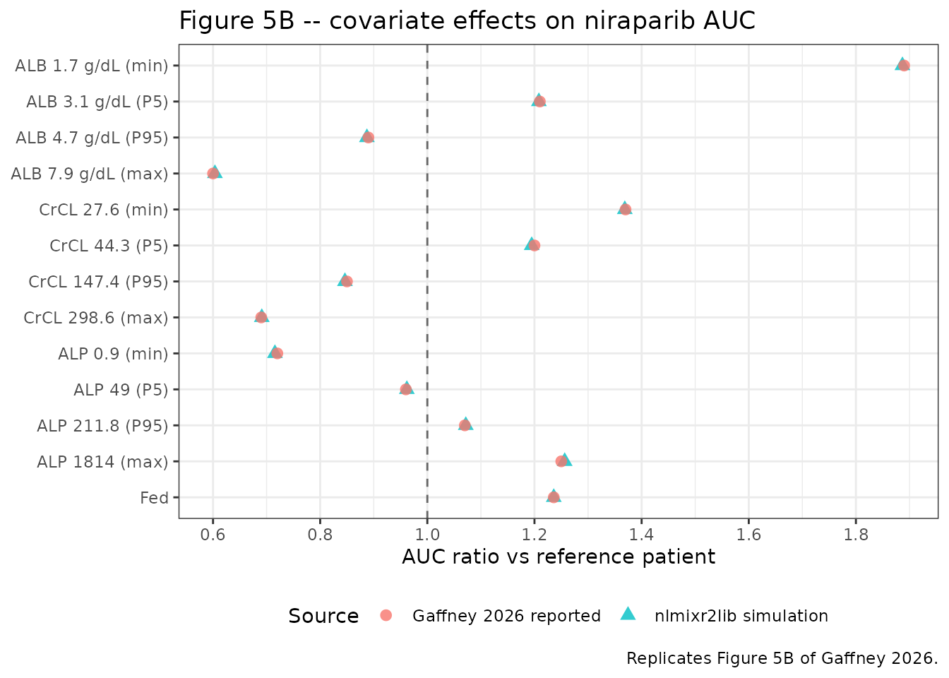
Terminal half-life and Tmax
The three-compartment disposition has analytic half-lives of 3.03, 34.0 and 136.0 h (eigenvalues of the rate-constant matrix at the typical values). NCA over the 1000 h window should recover the terminal phase.
micro <- tv
rate_matrix <- matrix(c(
  -(micro$kel + micro$k12 + micro$k13), micro$k21, micro$k31,
  micro$k12,                           -micro$k21, 0,
  micro$k13,                            0,         -micro$k31
), nrow = 3, byrow = TRUE)
analytic_hl <- sort(log(2) / -Re(eigen(rate_matrix)$values))

hl_nca <- scen_res$half.life[scen_res$scenario == "Reference"]
tmax_fasted <- scen_res$tmax[scen_res$scenario == "Reference"]
tmax_fed <- scen_res$tmax[scen_res$scenario == "Fed"]

tibble::tibble(
  Quantity = c("Terminal half-life (h)", "Tmax, fasted/unknown (h)",
               "Tmax, fed (h)"),
  Model = c(hl_nca, tmax_fasted, tmax_fed),
  `Analytic / expected` = c(max(analytic_hl), NA_real_, NA_real_)
) |>
knitr::kable(digits = 2, caption = "Terminal half-life and Tmax at typical values.")| Quantity | Model | Analytic / expected |
|---|---|---|
| Terminal half-life (h) | 134.75 | 136.02 |
| Tmax, fasted/unknown (h) | 3.45 | NA |
| Tmax, fed (h) | 6.40 | NA |
stopifnot(
  # NCA fits the terminal slope over a finite window, so allow 3%.
  abs(hl_nca - max(analytic_hl)) / max(analytic_hl) < 0.03,
  # Figure 4 shows the TABLET and HEPATIC pcVPC medians peaking within the
  # first few hours after dose; both typical Tmax values must sit in that band.
  tmax_fasted > 1.5, tmax_fasted < 6,
  # A 115% increase in MTT must move Tmax substantially later.
  tmax_fed > tmax_fasted + 1.5
)
Virtual cohort
Individual patient data are not public. The cohort below draws covariates from log-normal distributions matched to the percentiles the paper reports for Figure 5 (ALB, ALP, CrCL); body weight uses the 70 kg reference with an assumed 20% coefficient of variation, because the weight distribution lives in Supplementary Table S1, which is not in the open-access deposit.
# set.seed() seeds R's RNG for the covariate draws. It does NOT seed rxode2's
# simulation RNG, whose streams are partitioned per solver thread -- so the etas
# below differ between a 2-core CI runner and a 16-thread workstation. Every
# assertion downstream is written to hold for any cohort the model can produce.
set.seed(20260901)
rxode2::rxSetSeed(20260901)

n_per_arm <- 150

# sigma on the log scale that reproduces the reported 5th and 95th percentiles.
log_sd <- function(p05, p95) (log(p95) - log(p05)) / (2 * stats::qnorm(0.95))

make_arm <- function(n, fed, label, id_offset) {
  tibble::tibble(
    id           = id_offset + seq_len(n),
    arm          = label,
    FED          = fed,
    ALB          = 40    * exp(stats::rnorm(n, 0, log_sd(31, 47))),
    ALP          = 83    * exp(stats::rnorm(n, 0, log_sd(49, 211.8))),
    CRCL         = 82.37 * exp(stats::rnorm(n, 0, log_sd(44.3, 147.4))),
    WT           = 70    * exp(stats::rnorm(n, 0, 0.20)),
    # TABLET is the study that supplied the intensively sampled single-dose
    # data these profiles emulate, so its residual magnitude is selected.
    STUDY_NOVA   = 0, STUDY_QUADRA = 0, STUDY_PRIMA = 0,
    STUDY_TABLET = 1, STUDY_HEPATIC = 0
  )
}

cohort <- dplyr::bind_rows(
  make_arm(n_per_arm, 0, "Fasted/unknown", id_offset = 0L),
  make_arm(n_per_arm, 1, "Fed",            id_offset = 1000L)
)

cohort_events <- expand_events(cohort, seq(0, 48, by = 0.25))
stopifnot(!anyDuplicated(unique(cohort_events[, c("id", "time", "evid")])))
cohort_sim <- rxode2::rxSolve(mod, events = cohort_events, keep = "arm") |>
  as.data.frame()
#> ℹ parameter labels from comments will be replaced by 'label()'

stopifnot(max(cohort_sim$Cc, na.rm = TRUE) > 1)

# The residual-error multiplexer must select the TABLET magnitude for every
# record in this cohort. Deterministic given the study indicators.
stopifnot(isTRUE(all.equal(unique(cohort_sim$expSdCc), 0.324)))
# Comparable to Figure 4 of Gaffney 2026: simulated concentration percentiles
# over the first 48 h after a single 300 mg dose. Gaffney 2026 plots
# prediction-corrected VPCs against observed data that are not public, so this
# reproduces the shape and magnitude of the profile rather than the pcVPC
# itself.
cohort_sim |>
  # Drop only the pre-dose record so the log-scale axis has no zero.
  dplyr::filter(time != 0) |>
  dplyr::group_by(arm, time) |>
  dplyr::summarise(
    Q05 = stats::quantile(Cc, 0.05),
    Q50 = stats::median(Cc),
    Q95 = stats::quantile(Cc, 0.95),
    .groups = "drop"
  ) |>
  ggplot(aes(time, Q50)) +
  geom_ribbon(aes(ymin = Q05, ymax = Q95), alpha = 0.25) +
  geom_line(linewidth = 0.7) +
  facet_wrap(~arm) +
  scale_y_log10() +
  labs(x = "Hours after dose", y = "Niraparib concentration (ng/mL)",
       title = "Simulated 5th / 50th / 95th percentiles, single 300 mg dose",
       caption = "Comparable to Figure 4 of Gaffney 2026 (TABLET panel).") +
  theme_bw()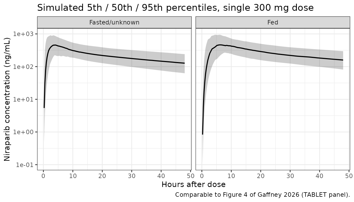
Cohort NCA by prandial state
cohort_conc <- cohort_sim |>
  dplyr::filter(!is.na(Cc)) |>
  dplyr::select(id, time, Cc, arm)

cohort_conc <- dplyr::bind_rows(
  cohort_conc,
  cohort_conc |> dplyr::distinct(id, arm) |> dplyr::mutate(time = 0, Cc = 0)
) |>
  dplyr::distinct(id, arm, time, .keep_all = TRUE) |>
  dplyr::arrange(id, time)

cohort_dose <- cohort_events |>
  dplyr::filter(evid == 1) |>
  dplyr::select(id, time, amt, arm)

cohort_nca <- PKNCA::pk.nca(PKNCA::PKNCAdata(
  PKNCA::PKNCAconc(cohort_conc, Cc ~ time | arm + id),
  PKNCA::PKNCAdose(cohort_dose, amt ~ time | arm + id),
  intervals = data.frame(start = 0, end = 48,
                         cmax = TRUE, tmax = TRUE, auclast = TRUE)
))

cohort_res <- as.data.frame(cohort_nca$result) |>
  dplyr::select(arm, id, PPTESTCD, PPORRES) |>
  tidyr::pivot_wider(names_from = PPTESTCD, values_from = PPORRES)

cohort_summary <- cohort_res |>
  dplyr::group_by(arm) |>
  dplyr::summarise(
    n = dplyr::n(),
    cmax_med = stats::median(cmax),
    tmax_med = stats::median(tmax),
    auc48_med = stats::median(auclast),
    .groups = "drop"
  )

cohort_summary |>
  dplyr::rename(
    "Prandial state"         = arm,
    "N"                      = n,
    "Median Cmax (ng/mL)"    = cmax_med,
    "Median Tmax (h)"        = tmax_med,
    "Median AUC0-48 (`ng*h/mL`)" = auc48_med
  ) |>
  knitr::kable(digits = 1, caption = paste(
    "Simulated single-dose NCA by prandial state (150 subjects per arm).",
    "Gaffney 2026 reports no NCA table, so these are descriptive; the",
    "quantitative gates are the typical-value checks above."
))| Prandial state | N | Median Cmax (ng/mL) | Median Tmax (h) | Median AUC0-48 (ng*h/mL) |
|---|---|---|---|---|
| Fasted/unknown | 150 | 478.5 | 3.2 | 10550.6 |
| Fed | 150 | 467.1 | 6.8 | 11647.5 |
The paper describes the prandial effects on exposure as “relatively minor” while MTT more than doubles when fed. Both are visible here: median Tmax moves several hours later, while median 48 h exposure changes modestly.
fed_row <- cohort_summary[cohort_summary$arm == "Fed", ]
fst_row <- cohort_summary[cohort_summary$arm == "Fasted/unknown", ]
stopifnot(nrow(fed_row) == 1L, nrow(fst_row) == 1L)

# A 115% increase in MTT is a large structural effect, not a near-zero one, so
# a median ordering with headroom is safe across cohorts. Realised gaps were
# 3.50 / 3.00 / 2.75 / 2.50 h at 1 / 2 / 4 / 16 solver threads, so 1 h leaves
# 1.5 h of headroom below the smallest observed value.
stopifnot(fed_row$tmax_med > fst_row$tmax_med + 1)

# "Relatively minor" effect on exposure: bound the MAGNITUDE of the median
# AUC0-48 change, not its sign. This is a descriptive cohort check, not the
# gate on the F1 food effect -- that gate is the deterministic "Fed" row of the
# published-ratio table above, where AUC(0-inf) reproduces 1.236 exactly. Over
# a truncated 48 h window the slower fed absorption partly offsets the higher
# F1, so the ratio lands near 1. Realised 1.104 / 1.203 / 1.080 / 1.205 at
# 1 / 2 / 4 / 16 solver threads; the 0.85-1.45 band leaves >0.23 of headroom on
# each side and still goes red on a sign-flipped fed effect on F1 (which would
# put the ratio near 0.68).
auc_ratio <- fed_row$auc48_med / fst_row$auc48_med
stopifnot(auc_ratio > 0.85, auc_ratio < 1.45)
Study-specific residual error
A separate additive-on-log-scale residual error was estimated for each pooled study. The model selects it from five binary study indicators, with PN001 as the reference level.
study_cols <- c("STUDY_NOVA", "STUDY_QUADRA", "STUDY_PRIMA",
                "STUDY_TABLET", "STUDY_HEPATIC")

study_subjects <- tibble::tibble(
  id    = 1:6,
  study = c("PN001", "NOVA", "QUADRA", "PRIMA", "TABLET", "HEPATIC"),
  ALB = 40, ALP = 83, CRCL = 82.37, WT = 70, FED = 0
)
for (j in seq_along(study_cols)) {
  study_subjects[[study_cols[j]]] <- as.numeric(study_subjects$id == j + 1L)
}

study_sim <- rxode2::rxSolve(
  rxode2::zeroRe(mod),
  events = expand_events(study_subjects, seq(0, 24, by = 1)),
  keep = "study", omega = NA
) |>
  as.data.frame()
#> ℹ parameter labels from comments will be replaced by 'label()'
#> Warning: No sigma parameters in the model
#> Warning: multi-subject simulation without without 'omega'

study_check <- study_sim |>
  dplyr::group_by(study) |>
  dplyr::summarise(model = unique(expSdCc), .groups = "drop") |>
  dplyr::left_join(
    tibble::tibble(
      study = c("PN001", "NOVA", "QUADRA", "PRIMA", "TABLET", "HEPATIC"),
      published = c(0.227, 0.350, 0.381, 0.451, 0.324, 0.146)
    ),
    by = "study"
  )

study_check |>
  dplyr::rename("Study" = study,
                "Model log-scale residual SD" = model,
                "Gaffney 2026 Table 3" = published) |>
  knitr::kable(digits = 3,
caption = "Study-specific residual-error selection.")| Study | Model log-scale residual SD | Gaffney 2026 Table 3 |
|---|---|---|
| HEPATIC | 0.146 | 0.146 |
| NOVA | 0.350 | 0.350 |
| PN001 | 0.227 | 0.227 |
| PRIMA | 0.451 | 0.451 |
| QUADRA | 0.381 | 0.381 |
| TABLET | 0.324 | 0.324 |
Assumptions and deviations
-
The transit rate constant is derived as
ktr = 3 / MTT, not4 / MTT. Table 3 reports MTT but no absorption rate constant, and the paper never writes the absorption ODEs out. The commonly used Savic (2007) parameterisation is quoted asMTT = (n + 1) / ktrforntransit compartments, which would givektr = 4 / 1.78 = 2.247 1/hhere. That reading was rejected for three reasons. (i) Savic’sn + 1counts first-order steps, not boxes – the dose lands in a dosing compartment and the chain runs to a separate absorption compartment, giving one more step than there are labelled transit compartments. Figure 3 has no such extra step: the dose arrow enters the first Transit box and the third Transit empties directly into Central, so the diagram has exactly threeKaarrows between the dose record and the central compartment. (ii) The mean of a sum of three exponential steps at ratektris3 / ktr, soMTT = 1.78 his self-consistent with the name only under this reading. (iii) The typical Tmax is 3.45 h under3 / MTTand 2.70 h under4 / MTT; the TABLET and HEPATIC pcVPC panels in Figure 4 show the medians peaking around 4-5 h (a mixture of fasted and fed records, whose typical Tmax values are 3.45 and 6.40 h under this reading), which the3 / MTTreading matches better. If the authors did in fact code the Savic(n + 1)form with three boxes, absorption in this file is 33% slower than theirs; exposure (AUC) is unaffected either way, since MTT does not enter the AUC. -
Albumin unit convention. The paper reports albumin
in the US convention g/dL and the canonical
ALBcolumn is SI g/L. The reference is therefore written as 40 g/L rather than 4 g/dL. Because albumin enters only as the ratio(ALB / 40), this is a pure relabelling with no effect on any coefficient – confirmed by the exact reproduction of all four published albumin AUC ratios. -
Creatinine clearance is not BSA-normalized. The
canonical
CRCLcolumn is documented in mL/min/1.73 m^2, but Gaffney 2026 reports raw creatinine clearance in mL/min (reference 82.37 mL/min) and does not name the estimating equation. The model’scovariateDatarecords the raw-mL/min convention. Raw mL/min is the convention used by mostCRCLmodels already in the library. - Q1/F. Table 3 reports 43.8 L/h and the Discussion quotes 43.5 L/h for the same parameter. The Table 3 value is used, being the parameter table.
- No off-diagonal IIV. The paper says alternative variance-covariance structures were investigated during covariate modelling, but Table 3 reports only the five diagonal IIV magnitudes as CV%, with no covariances or correlations. The diagonal form is encoded.
-
Residual error is encoded as
lnorm(). The Table 3 note states that “an additive residual error model on log-transformed concentrations was used”, which is exactly nlmixr2’s log-normal error structure with the SD on the log scale. The tabulated values (labelled “Res variability CV”) are taken as those log-scale SDs. -
PN001 is the residual-error reference level. The
paper gives six co-equal study-specific magnitudes with no reference.
Encoding them as five binary indicators plus a bare
expSdrequires nominating one; PN001 was chosen as the earliest study and the first row of both Table 1 and the Table 3 residual block. A record with all five indicators at 0 therefore receives the PN001 magnitude. - Supplementary Table S1 was not available. No supplementary material is deposited with PMC13185089, so the baseline demographic table (age, weight and race distributions) could not be read. The population metadata records the percentages quoted in the Results text instead, and the virtual cohort’s body-weight distribution is an assumption (70 kg median, 20% CV) rather than a transcription. The albumin, alkaline phosphatase and creatinine clearance distributions are anchored to published percentiles.
-
No published NCA table. Gaffney 2026 reports no
non-compartmental Cmax / Tmax / AUC summary, so there is no
ncaComparisonTable()comparison here. The published quantities that exist – the thirteen exposure ratios of Figure 5B, the total apparent volume of 1206 L, and the six residual-error magnitudes – are each gated above instead. -
Hepatic impairment is not a model covariate. Eight
patients in HEPATIC had moderate hepatic impairment, which the paper
names as too few to identify an effect.
STUDY_HEPATICis a study-membership indicator that selects a residual-error magnitude, not a hepatic-function covariate.