Indocyanine green whole-body PBPK in cirrhosis and hepatectomy (Koller 2021)
Source:vignettes/articles/Koller_2021_indocyanineGreen_pbpk.Rmd
Koller_2021_indocyanineGreen_pbpk.RmdThe model
Koller_2021_indocyanineGreen_pbpk is the whole-body
physiologically based pharmacokinetic model of indocyanine green (ICG)
that Koller, Grzegorzewski, Tautenhahn and Koenig (2021) built to
predict how liver cirrhosis and partial hepatectomy change the ICG
liver-function test. The authors distribute it as SBML (model version
1.0.0, the version used in the paper).
mod <- rxode2::rxode2(readModelDb("Koller_2021_indocyanineGreen_pbpk"))
mod$state
#>  [1] "depot_iv"     "venous"       "lung_plasma"  "arterial"     "rest_plasma"
#>  [6] "gut_plasma"   "portal"       "liver_plasma" "hepatic_vein" "liver"
#> [11] "bile"         "a_feces"
The 12 states are amounts in mg:
-
Intravenous input. The dose enters
depot_ivand empties into venous plasma at a first-order rate whose half-life equals the injection time (ti_icg= 5 s). An infusion is given as arateinto the same compartment. - Circulation. Venous plasma flows through the lung to arterial plasma, and from there to the gastrointestinal tract (then the portal vein), the hepatic artery and a lumped rest-of-body plasma pool. Portal and hepatic arterial blood perfuse liver plasma and drain through the hepatic vein. All transport is irreversible and proportional to blood flow. There is no tissue distribution outside the liver: ICG is highly protein-bound and stays in the vascular space.
- Liver. ICG is taken up from liver plasma into hepatocytes by saturable (Michaelis-Menten) transport, competitively inhibited by bilirubin, then exported into bile (Michaelis-Menten) and carried from bile to feces (first order). All three rates scale with the functional liver tissue volume.
-
Cirrhosis.
HEPFUNC_REL = 1 - f_cirrhosis. The paper’sf_cirrhosisremoves that fraction of parenchymal tissue and shunts that fraction of portal and hepatic arterial blood directly to the hepatic vein. -
Hepatectomy.
resection_rateremoves that fraction of liver volume. It is a fixed parameter inini(); supply aresection_ratecolumn in the event data to vary it per subject, since rxode2 lets a data column override a parameter of the same name.
Cc is venous plasma ICG in mg/L, the concentration from
which the paper computes ICG-R15, the plasma disappearance rate (PDR),
clearance and half-life. C_arterial,
C_hepatic_vein and the hepatic extraction ratio
ER are also returned. The model is deterministic: the
authors fitted one typical individual, so it has no between-subject
variability and a zero residual error.
Population
The model was parameterised on data curated from 29 clinical ICG
studies into the PK-DB database (Table 1). The five hepatic transport
parameters were fitted by weighted least squares to plasma, bile and
extraction-ratio time courses from 13 studies in healthy subjects (Table
1, ‘Fit’ column). All data in cirrhosis (Child-Turcotte-Pugh classes
A-C) and after partial hepatectomy were kept for validation. Doses were
intravenous boluses of 0.25-5.0 mg/kg (or a flat 10-20 mg) and constant
infusions of 0.08-2.0 mg/min. Study-specific body weights (58.2-83.4 kg,
where reported) were used, and 75 kg otherwise. The survival classifiers
of Section 3.5 used 141 Japanese hepatectomy patients (109 survivors, 32
non-survivors). The same information is in the model’s
population metadata.
Source trace
| Model element | Value | Source |
|---|---|---|
| Structure: circulation, liver, cirrhosis, hepatectomy | – | Section 3.1, Figure 1A-D |
| Rate laws and ODEs | – | Model archive version 1.0.0 (doi:10.5281/zenodo.5552405),
models/icg_body_flat.xml
|
covbw (COBW) |
0.8333 mL/s/kg | Table 2 (printed 0.83) |
hct, fblood
|
0.51, 0.02 | Table 2 |
fvbi, fvli, fvve,
fvar, fvpo, fvhv
|
0.00071, 0.021, 0.0587, 0.0184, 0.001, 0.001 L/kg | Table 2 |
fvgi, fvlu
|
0.0297, 0.0076 L/kg | Model archive; Table 2 prints 0.0171 and 0.0297 (see Errata) |
fqgi, fqh
|
0.19, 0.255 | Table 2 |
fqlu |
1 | Section 2.4 (“must be 1”) |
mr_icg, ti_icg
|
774.96 g/mol, 5 s | Table 2 |
icgim_vmax, icgim_km
|
0.0370 mmol/min/L, 0.0217 mmol/L | Table 2 (fitted) |
icgli2ca_vmax, icgli2ca_km
|
0.000944 mmol/min/L, 0.0124 mmol/L | Table 2 (fitted) |
icgli2bi_k |
0.000114 1/min | Table 2 (fitted; printed as LI__ICGLI2BI_Vmax) |
icgim_ki_bil |
0.02 mmol/L | Table 2 |
bil_ext |
0.01 mmol/L | Model archive (bilirubin initial concentration); Table 2 comment on ki_bil |
wt_ref |
75 kg | Table 2 (BW) |
f_cardiac_output, f_bloodflow,
f_oatp1b3, resection_rate
|
1, 1, 1, 0 | Table 2 (scan parameters) |
HEPFUNC_REL levels |
1, 0.59, 0.30, 0.18 | Section 3.3 / Figure 5E (f_cirrhosis 0, 0.41, 0.70, 0.82) |
| f_cirrhosis from pre-operative R15 | a = 0.312, b = 1.693, c = 0.861 | Section 2.6, Eq. 2 |
propSd |
0 (fixed) | Section 4.2 (one deterministic parameter set) |
Simulation helpers
# Observation grid (min): dense over the 15-s peak, then every 3 s to 60 min.
obs_grid <- c(seq(0, 1, by = 0.01), seq(1.05, 60, by = 0.05))

# One bolus per subject into depot_iv; observations on the venous state.
# `design` has one row per subject with columns id, dose_mg, WT,
# HEPFUNC_REL and resection_rate (plus any grouping columns).
make_bolus_events <- function(design, times = obs_grid) {
  dose <- design |>
    mutate(time = 0, amt = dose_mg, evid = 1L, cmt = "depot_iv")
  obs <- design |>
    tidyr::crossing(time = times) |>
    mutate(amt = 0, evid = 0L, cmt = "venous")
  bind_rows(dose, obs) |>
    arrange(id, time, desc(evid)) |>
    as.data.frame()
}

solve_icg <- function(model, events) {
  suppressWarnings(rxode2::rxSolve(
    model, events,
    atol = 1e-12, rtol = 1e-10, maxsteps = 1e6,
    addCov = TRUE, returnType = "data.frame"
  ))
}

# ICG parameters as defined in Section 2.5: R15 = C(15)/Cmax; kel from an
# exponential fit (here log-linear over 2-15 min, the window the paper leaves
# unstated); PDR = 100 * kel; clearance = dose / AUCinf; t1/2 = log(2) / kel.
icg_parameters <- function(sim, dose_col = "dose_mg") {
  sim |>
    group_by(id) |>
    summarise(
      dose = first(.data[[dose_col]]),
      cmax = max(Cc),
      c15 = Cc[which.min(abs(time - 15))],
      kel = -coef(stats::lm(log(Cc[time >= 2 & time <= 15]) ~
        time[time >= 2 & time <= 15]))[[2]],
      auc_last = sum(diff(time) * (head(Cc, -1) + tail(Cc, -1)) / 2),
      c_last = last(Cc),
      .groups = "drop"
    ) |>
    mutate(
      R15 = 100 * c15 / cmax,
      PDR = 100 * kel,
      CL = dose / (auc_last + c_last / kel),
      thalf = log(2) / kel
    )
}
Reproducing the deposited SBML model
The authors’ model archive runs in libroadrunner. The maintainers
solved icg_body_flat.xml from that archive in libroadrunner
2.10.0 for ten bolus scenarios and the three-rate infusion protocol of
Soons 1991 (Figure 2F). Venous and hepatic-venous concentrations at four
times per bolus scenario are embedded below. Both sides use the same
parameter values, so the difference is pure numerical error and a tight
bound is appropriate.
sbml_ref <- tibble::tribble(
  ~scenario, ~dose_mg, ~WT, ~f_cirrhosis, ~resection_rate, ~time, ~Cve, ~Chv,
  "bolus", 37.5, 75, 0.0, 0.0, 1, 10.8160604, 4.49266328,
  "bolus", 37.5, 75, 0.0, 0.0, 5, 4.65174835, 1.80059898,
  "bolus", 37.5, 75, 0.0, 0.0, 15, 0.531313557, 0.197981454,
  "bolus", 37.5, 75, 0.0, 0.0, 30, 0.0198995002, 0.00737997017,
  "bolus", 37.5, 75, 0.0, 0.5, 1, 11.6652288, 7.77982031,
  "bolus", 37.5, 75, 0.0, 0.5, 5, 7.10143694, 4.55016532,
  "bolus", 37.5, 75, 0.0, 0.5, 15, 1.91571152, 1.18619654,
  "bolus", 37.5, 75, 0.0, 0.5, 30, 0.250659873, 0.153416637,
  "bolus", 37.5, 75, 0.41, 0.0, 1, 11.6720007, 7.7893656,
  "bolus", 37.5, 75, 0.41, 0.0, 5, 7.1608226, 4.65623273,
  "bolus", 37.5, 75, 0.41, 0.0, 15, 2.04496546, 1.30904762,
  "bolus", 37.5, 75, 0.41, 0.0, 30, 0.302306494, 0.192500512,
  "bolus", 37.5, 75, 0.41, 0.5, 1, 12.1915844, 9.88329138,
  "bolus", 37.5, 75, 0.41, 0.5, 5, 9.14531346, 7.26994137,
  "bolus", 37.5, 75, 0.41, 0.5, 15, 4.3270626, 3.3914264,
  "bolus", 37.5, 75, 0.41, 0.5, 30, 1.34200475, 1.04219448,
  "bolus", 37.5, 75, 0.7, 0.0, 1, 12.3023596, 10.3155498,
  "bolus", 37.5, 75, 0.7, 0.0, 5, 9.62746633, 7.96057902,
  "bolus", 37.5, 75, 0.7, 0.0, 15, 5.16565356, 4.24865228,
  "bolus", 37.5, 75, 0.7, 0.0, 30, 1.99098912, 1.63150162,
  "bolus", 37.5, 75, 0.7, 0.5, 1, 12.5721501, 11.4362016,
  "bolus", 37.5, 75, 0.7, 0.5, 5, 10.8797365, 9.77429767,
  "bolus", 37.5, 75, 0.7, 0.5, 15, 7.52702389, 6.73389393,
  "bolus", 37.5, 75, 0.7, 0.5, 30, 4.24393487, 3.7805732,
  "bolus", 37.5, 75, 0.82, 0.0, 1, 12.5692848, 11.4090922,
  "bolus", 37.5, 75, 0.82, 0.0, 5, 10.8555347, 9.74141075,
  "bolus", 37.5, 75, 0.82, 0.0, 15, 7.50838301, 6.72306434,
  "bolus", 37.5, 75, 0.82, 0.0, 30, 4.27507933, 3.82000712,
  "bolus", 37.5, 75, 0.82, 0.5, 1, 12.7316044, 12.0947254,
  "bolus", 37.5, 75, 0.82, 0.5, 5, 11.6745314, 10.9708571,
  "bolus", 37.5, 75, 0.82, 0.5, 15, 9.39297171, 8.81270336,
  "bolus", 37.5, 75, 0.82, 0.5, 30, 6.71858224, 6.2913886,
  "bolus", 375.0, 75, 0.0, 0.0, 1, 118.453829, 86.784063,
  "bolus", 375.0, 75, 0.0, 0.0, 5, 74.8055509, 47.0302201,
  "bolus", 375.0, 75, 0.0, 0.0, 15, 13.2164623, 5.52789772,
  "bolus", 375.0, 75, 0.0, 0.0, 30, 0.529559975, 0.197324813,
  "bolus", 10.0, 60, 0.0, 0.0, 1, 3.59686395, 1.46604003,
  "bolus", 10.0, 60, 0.0, 0.0, 5, 1.55077089, 0.61251727,
  "bolus", 10.0, 60, 0.0, 0.0, 15, 0.186123009, 0.0726447403,
  "bolus", 10.0, 60, 0.0, 0.0, 30, 0.0076620108, 0.00298586311,
  "infusion", NA, 72, 0.0, 0.0, 20, 3.39066381, 1.24243116,
  "infusion", NA, 72, 0.0, 0.0, 40, 3.44033136, 1.26213546,
  "infusion", NA, 72, 0.0, 0.0, 60, 0.883848446, 0.317559712,
  "infusion", NA, 72, 0.0, 0.0, 80, 0.849445555, 0.30449646,
  "infusion", NA, 72, 0.0, 0.0, 100, 1.69355931, 0.611458774,
  "infusion", NA, 72, 0.0, 0.0, 120, 1.70514812, 0.615923011
)

bolus_design <- sbml_ref |>
  filter(scenario == "bolus") |>
  distinct(dose_mg, WT, f_cirrhosis, resection_rate) |>
  mutate(id = row_number(), HEPFUNC_REL = 1 - f_cirrhosis)
sim_bolus <- solve_icg(
  mod,
  make_bolus_events(select(bolus_design, -f_cirrhosis),
                    times = c(0, 1, 5, 15, 30))
) |>
  select(id, time, Cc, C_hepatic_vein)

# Soons 1991: 2.0, 0.5 and 1.0 mg/min, 40 min each, 72 kg.
soons_events <- bind_rows(
  data.frame(
    id = 1, time = c(0, 40, 80), amt = c(80, 20, 40), rate = c(2, 0.5, 1),
    evid = 1L, cmt = "depot_iv"
  ),
  data.frame(
    id = 1, time = seq(0, 120, by = 0.5), amt = 0, rate = 0,
    evid = 0L, cmt = "venous"
  )
) |>
  mutate(WT = 72, HEPFUNC_REL = 1, resection_rate = 0) |>
  arrange(time, desc(evid))
sim_soons <- solve_icg(mod, soons_events)

cmp_sbml <- bind_rows(
  sbml_ref |>
    filter(scenario == "bolus") |>
    inner_join(
      select(bolus_design, id, dose_mg, WT, f_cirrhosis, resection_rate),
      by = c("dose_mg", "WT", "f_cirrhosis", "resection_rate")
    ) |>
    inner_join(sim_bolus, by = c("id", "time")) |>
    select(-id),
  sbml_ref |>
    filter(scenario == "infusion") |>
    inner_join(select(sim_soons, time, Cc, C_hepatic_vein), by = "time")
) |>
  mutate(
    rel_venous = Cc / Cve - 1,
    rel_hepatic_vein = C_hepatic_vein / Chv - 1
  )

cmp_sbml |>
  group_by(scenario, dose_mg, WT, f_cirrhosis, resection_rate) |>
  summarise(
    `Max abs rel. diff, venous` = max(abs(rel_venous)),
    `Max abs rel. diff, hepatic vein` = max(abs(rel_hepatic_vein)),
    .groups = "drop"
  ) |>
  rename(
    "Scenario" = scenario, "Dose (mg)" = dose_mg, "WT (kg)" = WT,
    "f_cirrhosis" = f_cirrhosis, "Resection rate" = resection_rate
  ) |>
knitr::kable(digits = 10)| Scenario | Dose (mg) | WT (kg) | f_cirrhosis | Resection rate | Max abs rel. diff, venous | Max abs rel. diff, hepatic vein |
|---|---|---|---|---|---|---|
| bolus | 10.0 | 60 | 0.00 | 0.0 | 1.7e-09 | 1.0e-09 |
| bolus | 37.5 | 75 | 0.00 | 0.0 | 2.1e-09 | 1.9e-09 |
| bolus | 37.5 | 75 | 0.00 | 0.5 | 2.6e-09 | 2.4e-09 |
| bolus | 37.5 | 75 | 0.41 | 0.0 | 2.2e-09 | 3.2e-09 |
| bolus | 37.5 | 75 | 0.41 | 0.5 | 4.6e-09 | 1.7e-09 |
| bolus | 37.5 | 75 | 0.70 | 0.0 | 8.0e-10 | 2.2e-09 |
| bolus | 37.5 | 75 | 0.70 | 0.5 | 2.7e-09 | 3.6e-09 |
| bolus | 37.5 | 75 | 0.82 | 0.0 | 9.0e-10 | 1.1e-09 |
| bolus | 37.5 | 75 | 0.82 | 0.5 | 3.9e-09 | 2.9e-09 |
| bolus | 375.0 | 75 | 0.00 | 0.0 | 4.2e-09 | 2.0e-09 |
| infusion | NA | 72 | 0.00 | 0.0 | 2.2e-09 | 1.4e-09 |
stopifnot(
  nrow(cmp_sbml) == nrow(sbml_ref),
  max(abs(cmp_sbml$rel_venous)) < 1e-5,
  max(abs(cmp_sbml$rel_hepatic_vein)) < 1e-5
)
The nlmixr2lib translation reproduces the libroadrunner solution of the authors’ own SBML file to within solver tolerance in every scenario. These scenarios cover the four cirrhosis degrees, with and without 50% resection, a 10-fold dose that saturates hepatic uptake, a non-reference body weight, and a multi-rate infusion.
Mass balance
ICG is neither metabolised nor excreted renally, so every mg that
leaves depot_iv must be in a plasma pool, the liver, bile
or feces.
mb_events <- make_bolus_events(
  data.frame(id = 1, dose_mg = 37.5, WT = 75, HEPFUNC_REL = 1,
             resection_rate = 0),
  times = seq(0, 600, by = 10)
)
mb <- solve_icg(mod, mb_events) |>
  mutate(
    total = depot_iv + venous + lung_plasma + arterial + rest_plasma +
      gut_plasma + portal + liver_plasma + hepatic_vein + liver + bile +
      a_feces
  )
stopifnot(max(abs(mb$total - 37.5)) < 1e-6)

mb |>
  filter(time %in% c(10, 60, 600)) |>
  transmute(
    `Time (min)` = time,
    `Plasma (mg)` = venous + lung_plasma + arterial + rest_plasma +
      gut_plasma + portal + liver_plasma + hepatic_vein,
    `Hepatocytes (mg)` = liver, `Bile (mg)` = bile, `Feces (mg)` = a_feces
  ) |>
knitr::kable(digits = 3)| Time (min) | Plasma (mg) | Hepatocytes (mg) | Bile (mg) | Feces (mg) |
|---|---|---|---|---|
| 10 | 4.665 | 26.961 | 5.792 | 0.082 |
| 60 | 0.000 | 4.477 | 29.600 | 3.423 |
| 600 | 0.000 | 0.000 | 5.708 | 31.792 |
Plasma is cleared within the hour, while the dose passes more slowly through hepatocytes and bile. By 10 h about 85% has reached the feces. The paper calibrated these later steps only against biliary excretion data, and Figure 2H shows discrepancies at the two lower doses (Section 3.2). The plasma time course, the model’s stated focus (Section 4.2), is not affected by them because hepatic uptake is irreversible.
Cirrhosis and ICG-R15: the paper’s Eq. 2
Section 2.6 estimates an individual cirrhosis degree from a measured
pre-operative ICG-R15 with
f_cirrhosis = a * ln(b * R15) + c (a = 0.312, b = 1.693, c
= 0.861). The coefficients were fitted to the model’s own predicted
dependency of R15 on f_cirrhosis (Figure 4C). So Eq. 2 must
invert this model’s R15 curve.
f_grid <- c(0, 0.1, 0.2, 0.3, 0.41, 0.5, 0.6, 0.7, 0.82, 0.9)
cirr_design <- data.frame(
  id = seq_along(f_grid), f_cirrhosis = f_grid, dose_mg = 37.5, WT = 75,
  HEPFUNC_REL = 1 - f_grid, resection_rate = 0
)
cirr_par <- solve_icg(mod, make_bolus_events(select(cirr_design, -f_cirrhosis))) |>
  left_join(select(cirr_design, id, dose_mg), by = "id") |>
  icg_parameters() |>
  left_join(select(cirr_design, id, f_cirrhosis), by = "id") |>
  mutate(f_eq2 = 0.312 * log(1.693 * R15 / 100) + 0.861)

cirr_par |>
  select(f_cirrhosis, R15, PDR, CL, thalf, f_eq2) |>
  rename(
    "f_cirrhosis" = f_cirrhosis, "ICG-R15 (%)" = R15,
    "ICG-PDR (%/min)" = PDR, "Clearance (L/min)" = CL,
    "t1/2 (min)" = thalf, "f_cirrhosis from Eq. 2" = f_eq2
  ) |>
knitr::kable(digits = 3)| f_cirrhosis | ICG-R15 (%) | ICG-PDR (%/min) | Clearance (L/min) | t1/2 (min) | f_cirrhosis from Eq. 2 |
|---|---|---|---|---|---|
| 0.00 | 3.694 | 21.609 | 0.598 | 3.208 | -0.004 |
| 0.10 | 5.142 | 19.359 | 0.538 | 3.581 | 0.099 |
| 0.20 | 7.143 | 17.122 | 0.479 | 4.048 | 0.202 |
| 0.30 | 9.901 | 14.899 | 0.419 | 4.652 | 0.304 |
| 0.41 | 14.141 | 12.474 | 0.353 | 5.557 | 0.415 |
| 0.50 | 18.884 | 10.506 | 0.299 | 6.597 | 0.505 |
| 0.60 | 25.967 | 8.341 | 0.239 | 8.310 | 0.605 |
| 0.70 | 35.577 | 6.201 | 0.179 | 11.177 | 0.703 |
| 0.82 | 51.618 | 3.676 | 0.107 | 18.858 | 0.819 |
| 0.90 | 65.875 | 2.023 | 0.059 | 34.264 | 0.895 |
Eq. 2 recovers the input cirrhosis degree to within 0.01 across 0-0.9. This is an independent check that the extracted model is the one the paper ran. It also checks the healthy reference individual: R15 of about 3.7%, PDR of about 21.6 %/min and clearance of about 0.6 L/min, all inside the usual clinical normal ranges.
Figure 4A-D: shunts, tissue loss and cirrhosis
The paper separates the two components of cirrhosis. The maintainers
reproduce this by switching one component off in the model with
rxode2::model().
mod_shunt_only <- mod |> rxode2::model(f_tissue_loss <- 0)
mod_tissue_only <- mod |> rxode2::model(f_shunts <- 0)

f_scan <- seq(0, 0.9, by = 0.05)
scan_design <- data.frame(
  id = seq_along(f_scan), f = f_scan, dose_mg = 37.5, WT = 75,
  HEPFUNC_REL = 1 - f_scan, resection_rate = 0
)
scan_ev <- make_bolus_events(scan_design)
fig4 <- bind_rows(
  solve_icg(mod, scan_ev) |> mutate(component = "Cirrhosis (both)"),
  solve_icg(mod_shunt_only, scan_ev) |> mutate(component = "Shunts only"),
  solve_icg(mod_tissue_only, scan_ev) |> mutate(component = "Tissue loss only")
) |>
  left_join(select(scan_design, id, dose_mg, f), by = "id") |>
  group_by(component) |>
  group_modify(~ icg_parameters(.x) |>
    left_join(select(scan_design, id, f), by = "id")) |>
  ungroup()

fig4 |>
  tidyr::pivot_longer(c(CL, PDR, R15, thalf), names_to = "parameter") |>
  mutate(parameter = factor(
    parameter,
    levels = c("CL", "PDR", "R15", "thalf"),
    labels = c("Clearance (L/min)", "PDR (%/min)", "R15 (%)", "t1/2 (min)")
  )) |>
  ggplot(aes(f, value, colour = component)) +
  geom_line() +
  geom_point(size = 1) +
  facet_wrap(~parameter, scales = "free_y") +
  labs(x = "Fraction (f_shunts, f_tissue_loss or f_cirrhosis)", y = NULL,
       colour = NULL) +
  theme_bw() +
  theme(legend.position = "bottom")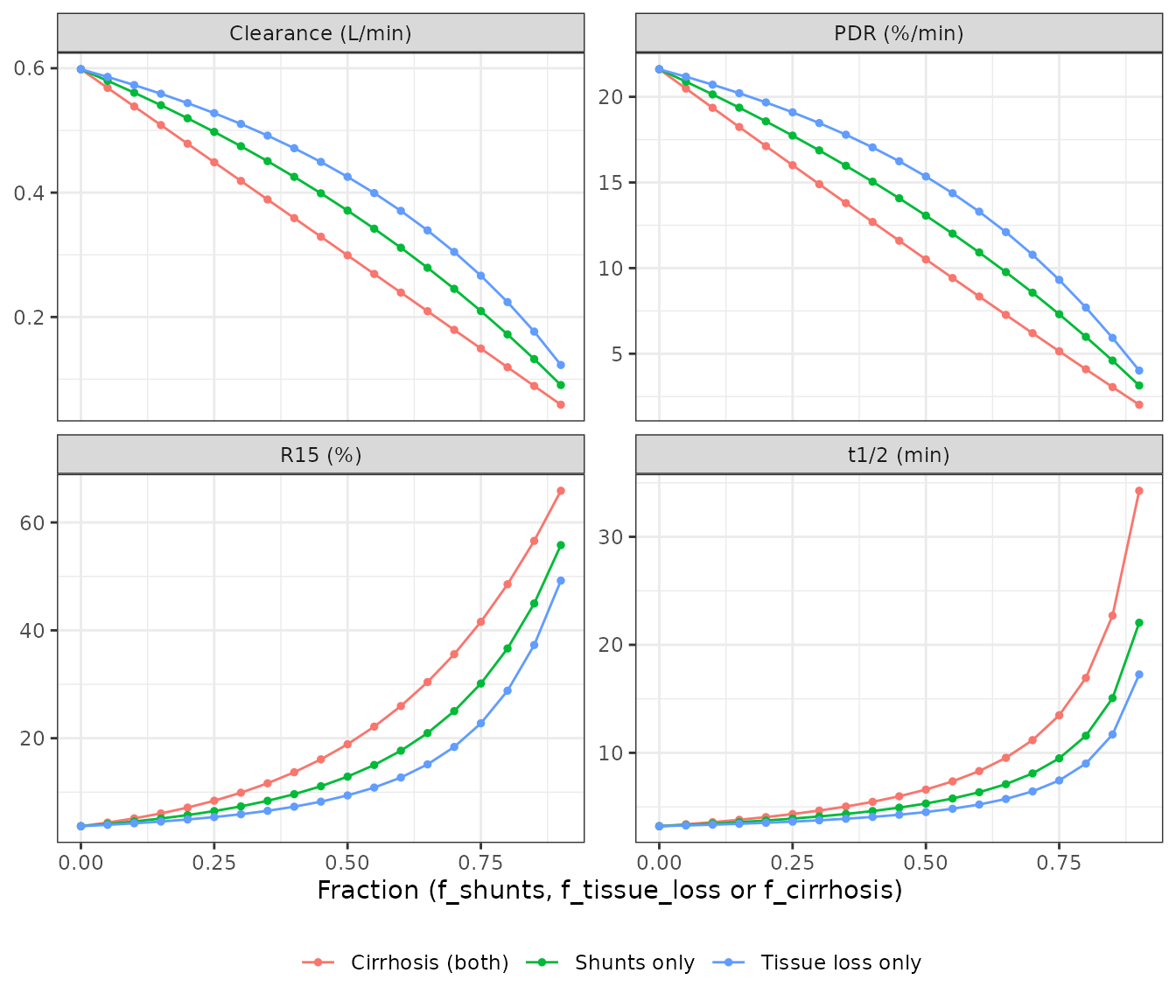
Replicates Figure 4A-D of Koller 2021.
at_half <- fig4 |> filter(abs(f - 0.5) < 1e-9)
cl_half <- setNames(at_half$CL, at_half$component)
stopifnot(
  # "The loss of a fraction of functional liver tissue appears to have a
  # smaller effect on ICG pharmacokinetic parameters than shunting of an
  # equal fraction of blood past the liver."
  cl_half[["Tissue loss only"]] > cl_half[["Shunts only"]],
  # Combined cirrhosis lowers clearance more than either component alone.
  cl_half[["Cirrhosis (both)"]] < cl_half[["Shunts only"]]
)
Figure 7: partial hepatectomy under cirrhosis
This is the central application. Resection rate is scanned from 0 to 0.9 on the paper’s 20-point grid for control and the three cirrhosis degrees mapped from Child-Turcotte-Pugh classes (Figure 5E).
cirrhosis_levels <- c(
  "Control" = 0, "Mild cirrhosis" = 0.41,
  "Moderate cirrhosis" = 0.70, "Severe cirrhosis" = 0.82
)
resect_grid <- seq(0, 0.9, length.out = 20)
fig7_design <- tidyr::crossing(
  group = factor(names(cirrhosis_levels), levels = names(cirrhosis_levels)),
  resection_rate = resect_grid
) |>
  mutate(
    id = row_number(),
    f_cirrhosis = unname(cirrhosis_levels[as.character(group)]),
    HEPFUNC_REL = 1 - f_cirrhosis, dose_mg = 37.5, WT = 75
  )
fig7_ev <- make_bolus_events(select(fig7_design, -group, -f_cirrhosis))
fig7 <- solve_icg(mod, fig7_ev) |>
  select(-resection_rate) |>
  left_join(select(fig7_design, id, dose_mg), by = "id") |>
  icg_parameters() |>
  left_join(select(fig7_design, id, group, resection_rate), by = "id")

fig7 |>
  tidyr::pivot_longer(c(CL, PDR, R15, thalf), names_to = "parameter") |>
  mutate(parameter = factor(
    parameter,
    levels = c("CL", "PDR", "R15", "thalf"),
    labels = c("Clearance (L/min)", "PDR (%/min)", "R15 (%)", "t1/2 (min)")
  )) |>
  ggplot(aes(resection_rate, value, colour = group)) +
  geom_line() +
  geom_point(size = 1) +
  facet_wrap(~parameter, scales = "free_y") +
  scale_colour_manual(values = c("black", "blue", "purple", "red")) +
  labs(x = "Resection rate", y = NULL, colour = NULL) +
  theme_bw() +
  theme(legend.position = "bottom")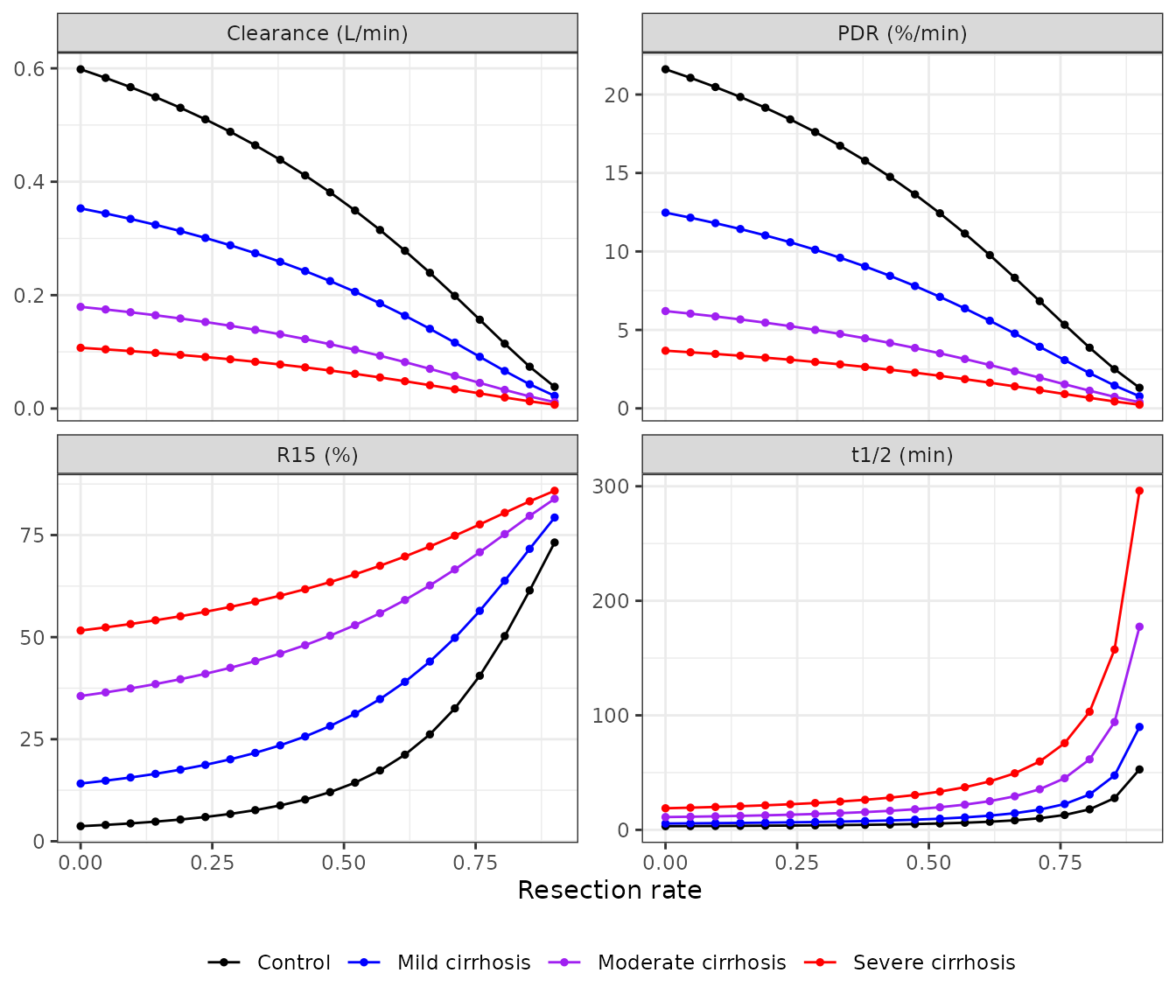
Replicates Figure 7A-D of Koller 2021.
The maintainers digitised markers from the published Figure 7A-C (reading precision about +/-1% of each axis range). The simulated curves are compared against them below. The same comparison is repeated with a counterfactual model in which the liver-plasma bilirubin concentration is held at 0.01 mmol/L regardless of resection. The Errata explain why that counterfactual is not the model the paper ran.
fig7_digitised <- tibble::tribble(
  ~group, ~resection_rate, ~panel, ~value,
  "Control", 0, "CL", 0.601,
  "Mild cirrhosis", 0, "CL", 0.360,
  "Moderate cirrhosis", 0, "CL", 0.181,
  "Severe cirrhosis", 0, "CL", 0.112,
  "Control", 0, "R15", 3.8,
  "Mild cirrhosis", 0, "R15", 13.8,
  "Moderate cirrhosis", 0, "R15", 35.5,
  "Severe cirrhosis", 0, "R15", 50.6,
  "Control", resect_grid[12], "R15", 14.5,
  "Control", resect_grid[14], "R15", 21.4,
  "Control", resect_grid[18], "R15", 50.5,
  "Control", resect_grid[20], "R15", 73.4,
  "Severe cirrhosis", resect_grid[20], "R15", 86.0,
  "Control", resect_grid[20], "CL", 0.039
)

# Counterfactual: bilirubin concentration fixed at bil_ext.
mod_bil_const <- mod |> rxode2::model(bil_li <- bil_ext)
fig7_const <- solve_icg(mod_bil_const, fig7_ev) |>
  select(-resection_rate) |>
  left_join(select(fig7_design, id, dose_mg), by = "id") |>
  icg_parameters() |>
  left_join(select(fig7_design, id, group, resection_rate), by = "id")

lookup_fig7 <- function(sim, grp, rs, panel) {
  row <- sim[as.character(sim$group) == grp &
    abs(sim$resection_rate - rs) < 1e-9, ]
  row[[panel]]
}
fig7_cmp <- fig7_digitised |>
  rowwise() |>
  mutate(
    model = lookup_fig7(fig7, group, resection_rate, panel),
    counterfactual = lookup_fig7(fig7_const, group, resection_rate, panel)
  ) |>
  ungroup() |>
  mutate(axis_range = ifelse(panel == "R15", 90, 0.6))

fig7_cmp |>
  select(-axis_range) |>
  rename(
    "Group" = group, "Resection rate" = resection_rate, "Panel" = panel,
    "Digitised" = value, "Model" = model,
    "Constant-bilirubin counterfactual" = counterfactual
  ) |>
knitr::kable(digits = 3)| Group | Resection rate | Panel | Digitised | Model | Constant-bilirubin counterfactual |
|---|---|---|---|---|---|
| Control | 0.000 | CL | 0.601 | 0.598 | 0.598 |
| Mild cirrhosis | 0.000 | CL | 0.360 | 0.353 | 0.353 |
| Moderate cirrhosis | 0.000 | CL | 0.181 | 0.179 | 0.179 |
| Severe cirrhosis | 0.000 | CL | 0.112 | 0.107 | 0.107 |
| Control | 0.000 | R15 | 3.800 | 3.694 | 3.694 |
| Mild cirrhosis | 0.000 | R15 | 13.800 | 14.141 | 14.141 |
| Moderate cirrhosis | 0.000 | R15 | 35.500 | 35.577 | 35.577 |
| Severe cirrhosis | 0.000 | R15 | 50.600 | 51.618 | 51.618 |
| Control | 0.521 | R15 | 14.500 | 14.359 | 9.952 |
| Control | 0.616 | R15 | 21.400 | 21.206 | 13.391 |
| Control | 0.805 | R15 | 50.500 | 50.258 | 29.520 |
| Control | 0.900 | R15 | 73.400 | 73.186 | 49.185 |
| Severe cirrhosis | 0.900 | R15 | 86.000 | 85.854 | 80.417 |
| Control | 0.900 | CL | 0.039 | 0.038 | 0.123 |
stopifnot(
  # Every digitised point is matched to within 3% of the axis range.
  all(abs(fig7_cmp$model - fig7_cmp$value) / fig7_cmp$axis_range < 0.03),
  # The counterfactual misses control R15 at 80% resection by > 10 points.
  with(
    subset(fig7_cmp, group == "Control" & panel == "R15" &
      abs(resection_rate - resect_grid[18]) < 1e-9),
    value - counterfactual > 10
  )
)
The model reproduces every digitised point of Figure 7. The counterfactual agrees at zero resection, where the two models are identical, but falls far below the published curve as resection increases.
Figure 8D: predicted post-operative ICG-R15
The PBPK1 classifier (Section 3.5) first estimates each patient’s
f_cirrhosis from their measured pre-operative R15 with Eq.
2. It then predicts post-operative R15 from that cirrhosis degree and
the planned resection rate. Figure 8B places the useful cutoffs at about
20% (no deaths below it) and 35-40% (the balanced-accuracy optimum). The
support vector classifiers themselves were trained on patient data and
publish no coefficients, so they are not part of the model. The PBPK
prediction step is reproduced here on a coarse grid.
grid8 <- tidyr::crossing(
  f_cirrhosis = seq(0, 0.8, by = 0.1),
  resection_rate = seq(0, 0.8, by = 0.1)
) |>
  mutate(id = row_number(), HEPFUNC_REL = 1 - f_cirrhosis, dose_mg = 37.5,
         WT = 75)
fig8 <- solve_icg(
  mod,
  make_bolus_events(select(grid8, -f_cirrhosis),
                    times = c(seq(0, 1, by = 0.01), 2, 15))
) |>
  group_by(id) |>
  summarise(R15 = 100 * Cc[time == 15] / max(Cc), .groups = "drop") |>
  left_join(grid8, by = "id")

ggplot(fig8, aes(resection_rate, f_cirrhosis, fill = R15)) +
  geom_tile() +
  geom_contour(aes(z = R15), breaks = c(20, 40), colour = "white") +
  scale_fill_viridis_c(name = "Predicted\npost-op R15 (%)") +
  labs(x = "Resection rate", y = "f_cirrhosis") +
  theme_bw()
#> Warning: The following aesthetics were dropped during statistical transformation: fill.
#> ℹ This can happen when ggplot fails to infer the correct grouping structure in
#>   the data.
#> ℹ Did you forget to specify a `group` aesthetic or to convert a numerical
#>   variable into a factor?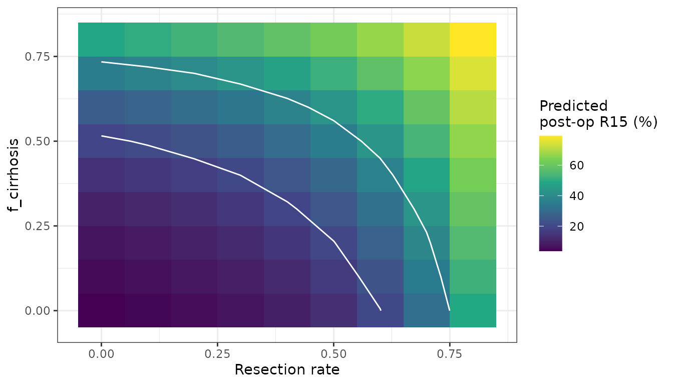
Replicates the structure of Figure 8D of Koller 2021 (white contours at 20% and 40%).
# Worked PBPK1 example: pre-operative R15 = 10%, planned 60% resection.
r15_preop <- 0.10
f_est <- 0.312 * log(1.693 * r15_preop) + 0.861
example <- solve_icg(
  mod,
  make_bolus_events(
    data.frame(id = 1:2, dose_mg = 37.5, WT = 75, HEPFUNC_REL = 1 - f_est,
               resection_rate = c(0, 0.6)),
    times = c(seq(0, 1, by = 0.01), 2, 15)
  )
) |>
  group_by(id) |>
  summarise(R15 = 100 * Cc[time == 15] / max(Cc), .groups = "drop")
data.frame(
  quantity = c("Estimated f_cirrhosis", "Model pre-operative R15 (%)",
               "Predicted post-operative R15 (%)"),
  value = c(f_est, example$R15)
) |>
  rename("Quantity" = quantity, "Value" = value) |>
knitr::kable(digits = 3)| Quantity | Value |
|---|---|
| Estimated f_cirrhosis | 0.307 |
| Model pre-operative R15 (%) | 10.125 |
| Predicted post-operative R15 (%) | 32.059 |
Dose dependency (Figure 3)
Section 3.2 reports that “a dose-dependency of the ICG parameters can only be observed if the ICG dose exceeds 100 mg”. Hepatic uptake saturates only at high doses.
dose_grid <- c(5, 10, 20, 37.5, 50, 100, 200, 375, 500)
dose_design <- data.frame(
  id = seq_along(dose_grid), dose_mg = dose_grid, WT = 75, HEPFUNC_REL = 1,
  resection_rate = 0
)
dose_par <- solve_icg(mod, make_bolus_events(dose_design)) |>
  left_join(select(dose_design, id, dose_mg), by = "id") |>
  icg_parameters()

dose_par |>
  select(dose, R15, PDR, CL, thalf) |>
  rename("Dose (mg)" = dose, "ICG-R15 (%)" = R15, "ICG-PDR (%/min)" = PDR,
         "Clearance (L/min)" = CL, "t1/2 (min)" = thalf) |>
knitr::kable(digits = 3)| Dose (mg) | ICG-R15 (%) | ICG-PDR (%/min) | Clearance (L/min) | t1/2 (min) |
|---|---|---|---|---|
| 5.0 | 3.482 | 21.877 | 0.616 | 3.168 |
| 10.0 | 3.513 | 21.838 | 0.614 | 3.174 |
| 20.0 | 3.576 | 21.757 | 0.608 | 3.186 |
| 37.5 | 3.694 | 21.609 | 0.598 | 3.208 |
| 50.0 | 3.785 | 21.497 | 0.591 | 3.224 |
| 100.0 | 4.210 | 20.993 | 0.560 | 3.302 |
| 200.0 | 5.421 | 19.650 | 0.496 | 3.527 |
| 375.0 | 9.167 | 16.180 | 0.396 | 4.284 |
| 500.0 | 13.503 | 13.305 | 0.341 | 5.210 |
pdr_at <- function(d) dose_par$PDR[dose_par$dose == d]
stopifnot(
  abs(pdr_at(100) / pdr_at(10) - 1) < 0.05,
  pdr_at(500) / pdr_at(10) < 0.8
)
PDR changes by less than 5% between 10 and 100 mg (the clinical dose is 20-35 mg) and falls clearly at higher doses, as Figure 3A-D shows.
Figure 2F: three-rate infusion (Soons 1991)
ggplot(sim_soons, aes(time, Cc)) +
  geom_line() +
  geom_vline(xintercept = c(40, 80), linetype = "dashed", colour = "grey50") +
  labs(x = "Time (min)", y = "Venous ICG (mg/L)") +
  theme_bw()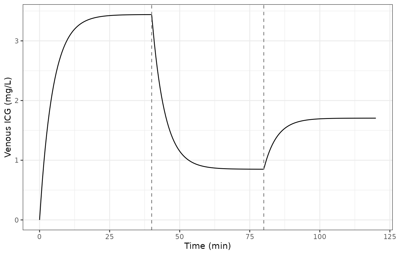
css <- sim_soons |> filter(time %in% c(35, 40, 75, 80, 115, 120))
stopifnot(
  # "the plasma concentration reaches steady state quickly after each change
  # in the infusion rate": the last 5 min of each 40-min step are flat.
  abs(css$Cc[2] / css$Cc[1] - 1) < 0.01,
  abs(css$Cc[4] / css$Cc[3] - 1) < 0.01,
  abs(css$Cc[6] / css$Cc[5] - 1) < 0.01
)
Replicates Figure 2F of Koller 2021 (2.0, 0.5 and 1.0 mg/min, 40 min each).
Non-compartmental analysis
PKNCA is run on a 0.5 mg/kg bolus (37.5 mg at 75 kg) in the four cirrhosis groups. The paper prints no NCA table, so the reference values are clearance and PDR digitised from Figure 7A-B at zero resection (PDR = 100 * lambda.z).
nca_design <- data.frame(
  id = 1:4, treatment = names(cirrhosis_levels),
  HEPFUNC_REL = 1 - unname(cirrhosis_levels), dose_mg = 37.5, WT = 75,
  resection_rate = 0
)
nca_sim <- solve_icg(
  mod,
  make_bolus_events(select(nca_design, -treatment),
                    times = c(obs_grid, seq(62, 240, by = 2)))
) |>
  left_join(select(nca_design, id, treatment), by = "id")

# Sample each group only while ICG is well above the solver's absolute
# tolerance: a healthy liver clears ICG to ~1e-12 mg/L by 4 h, where
# numerical noise would otherwise enter the terminal-phase fit.
nca_end <- c("Control" = 60, "Mild cirrhosis" = 120,
             "Moderate cirrhosis" = 240, "Severe cirrhosis" = 240)
conc_data <- nca_sim |>
  filter(!is.na(Cc), time <= nca_end[treatment]) |>
  select(id, treatment, time, Cc) |>
  as.data.frame()
dose_data <- nca_design |>
  mutate(time = 0) |>
  select(id, treatment, time, dose_mg) |>
  as.data.frame()

o_conc <- PKNCA::PKNCAconc(conc_data, Cc ~ time | treatment + id)
o_dose <- PKNCA::PKNCAdose(dose_data, dose_mg ~ time | treatment + id)
nca_res <- PKNCA::pk.nca(PKNCA::PKNCAdata(
  o_conc, o_dose,
  intervals = data.frame(
    start = 0, end = Inf, cmax = TRUE, tmax = TRUE, aucinf.obs = TRUE,
    cl.obs = TRUE, half.life = TRUE, lambda.z = TRUE
  )
))

nca_wide <- as.data.frame(nca_res$result) |>
  filter(PPTESTCD %in% c("cmax", "tmax", "aucinf.obs", "cl.obs",
                         "half.life", "lambda.z")) |>
  select(treatment, PPTESTCD, PPORRES) |>
  tidyr::pivot_wider(names_from = PPTESTCD, values_from = PPORRES)
nca_wide |>
  rename("Group" = treatment, "Cmax (mg/L)" = cmax, "tmax (min)" = tmax,
         "AUCinf (mg*min/L)" = aucinf.obs, "CL (L/min)" = cl.obs,
         "t1/2 (min)" = half.life, "lambda.z (1/min)" = lambda.z) |>
knitr::kable(digits = 4)| Group | Cmax (mg/L) | tmax (min) | lambda.z (1/min) | t1/2 (min) | AUCinf (mg*min/L) | CL (L/min) |
|---|---|---|---|---|---|---|
| Control | 14.3814 | 0.24 | 0.2188 | 3.1684 | 62.6752 | 0.5983 |
| Mild cirrhosis | 14.4612 | 0.25 | 0.1276 | 5.4341 | 106.2237 | 0.3530 |
| Moderate cirrhosis | 14.5196 | 0.26 | 0.0644 | 10.7638 | 208.8987 | 0.1795 |
| Severe cirrhosis | 14.5462 | 0.26 | 0.0384 | 18.0653 | 348.1584 | 0.1077 |
published <- tibble::tribble(
  ~treatment, ~cl.obs, ~lambda.z,
  "Control", 0.601, 0.217,
  "Mild cirrhosis", 0.360, 0.129,
  "Moderate cirrhosis", 0.181, 0.0633,
  "Severe cirrhosis", 0.112, 0.0388
)
cmp <- nlmixr2lib::ncaComparisonTable(
  simulated = as.data.frame(nca_res$result) |>
    select(treatment, PPTESTCD, PPORRES),
  reference = published,
  by = "treatment",
  params = c("cl.obs", "lambda.z"),
  units = c(cl.obs = "L/min", lambda.z = "1/min"),
  tolerance_pct = 20
)
cmp |>
  rename("Group" = treatment) |>
  knitr::kable(caption = paste(
    "Simulated NCA versus values digitised from Koller 2021 Figure 7A-B",
    "(resection rate 0). * differs by more than 20%."
))| NCA parameter | Group | Reference | Simulated | % diff |
|---|---|---|---|---|
| λz (1/min) | Control | 0.217 | 0.219 | +0.8% |
| λz (1/min) | Mild cirrhosis | 0.129 | 0.128 | -1.1% |
| λz (1/min) | Moderate cirrhosis | 0.0633 | 0.0644 | +1.7% |
| λz (1/min) | Severe cirrhosis | 0.0388 | 0.0384 | -1.1% |
| CL/F (L/min) | Control | 0.601 | 0.598 | -0.4% |
| CL/F (L/min) | Mild cirrhosis | 0.36 | 0.353 | -1.9% |
| CL/F (L/min) | Moderate cirrhosis | 0.181 | 0.18 | -0.8% |
| CL/F (L/min) | Severe cirrhosis | 0.112 | 0.108 | -3.8% |
# Measured differences are -0.4% to -3.8% (clearance) and within 2%
# (lambda.z); the digitisation itself is good to about +/-2%.
nca_cl <- setNames(nca_wide$cl.obs, nca_wide$treatment)
nca_lz <- setNames(nca_wide$lambda.z, nca_wide$treatment)
stopifnot(
  all(abs(nca_cl[published$treatment] / published$cl.obs - 1) < 0.1),
  all(abs(nca_lz[published$treatment] / published$lambda.z - 1) < 0.1)
)
PKNCA clearance and terminal rate constant both agree with the values
digitised from Figure 7A-B, to within a few percent in every group. The
disappearance is effectively mono-exponential after the first minute, so
the automatic terminal window and the paper’s unstated fitting window
give nearly the same rate. PKNCA labels clearance CL/F; for
this intravenous dose it is the systemic clearance,
Dose / AUCinf.
Assumptions and deviations / Errata
-
Rate laws come from the authors’ model archive. The
paper describes the structure (Section 3.1, Figure 1) and lists every
parameter (Table 2) but prints no rate laws. They were taken from
models/icg_body_flat.xmlof model version 1.0.0 (doi:10.5281/zenodo.5552405), which Section 3.1 names as the version used. The Zenodo archive is byte-identical to the GitHub release tag1.0.0(Oct 2021). The flat SBML reproduces the paper’s own Eq. 2 curve and Figure 7 (see above), which confirms that it is the as-run model. -
Two Table 2 fractional volumes disagree with the
archive. Table 2 prints
FVgi = 0.0171andFVlu = 0.0297L/kg; the archive hasFVgi = 0.0297andFVlu = 0.0076. The Table 2 lung value is the archive’s gut value, which looks like a transcription slip. The as-run archive values are used. The choice is immaterial, as the check below shows: gut and lung enter the ICG model only through their small plasma volumes and through the rest-of-body remainder.
mod_table2 <- mod |> rxode2::ini(fvgi = 0.0171, fvlu = 0.0297)
#> ℹ change initial estimate of `fvgi` to `0.0171`
#> ℹ change initial estimate of `fvlu` to `0.0297`
fv_par <- bind_rows(
  solve_icg(mod, make_bolus_events(cirr_design)) |> mutate(variant = "archive"),
  solve_icg(mod_table2, make_bolus_events(cirr_design)) |>
    mutate(variant = "Table 2")
) |>
  left_join(select(cirr_design, id, dose_mg), by = "id") |>
  group_by(variant) |>
  group_modify(~ icg_parameters(.x)) |>
  ungroup() |>
  select(variant, id, R15, PDR, CL) |>
  tidyr::pivot_wider(names_from = variant, values_from = c(R15, PDR, CL))
stopifnot(
  max(abs(fv_par$`R15_Table 2` / fv_par$R15_archive - 1)) < 0.01,
  max(abs(fv_par$`CL_Table 2` / fv_par$CL_archive - 1)) < 0.01
)-
Bilirubin behaves as it did in the paper’s simulations, not
as a fixed concentration. In the archive, liver-plasma
bilirubin is a reaction-free species with an initial concentration of
0.01 mmol/L, which suggests a constant concentration. In the paper’s
simulator, however, changing body weight or resection rate kept the
bilirubin amount at its reference value. Shrinking the
liver-plasma volume therefore raised the concentration by
(75 / WT) / (1 - resection_rate), strengthening the competitive inhibition of ICG uptake. The maintainers established this from Figure 7: the as-run form matches every digitised point, while a constant concentration misses control R15 at 80% resection by more than 10 percentage points (section above). The same behaviour is present in the body-weight-adjusted calibration fits (Section 3.2), so the fitted Vmax and Km absorb it. The model encodes the as-run form asbil_li <- bil_ext * vli_plasma_ref / vli_plasma, withvli_plasma_refevaluated atwt_ref= 75 kg and no resection. Cirrhosis does not change liver-plasma volume and is unaffected. For a constant-bilirubin variant, usemod |> rxode2::model(bil_li <- bil_ext). -
Axis unit in Figure 7A. The clearance axis is
labelled “ml/min”, but the plotted values (0.6 for a healthy liver) are
L/min: 600 mL/min, as the model gives with
Dose / AUCinf. -
Full-precision fitted values. Table 2 prints the
five fitted transport parameters to three significant figures. The
archive’s full-precision values are used; each rounds to the Table 2
entry.
COBWis printed as 0.83 and is 5/6 mL/s/kg in the archive, giving a cardiac output of 3.75 L/min at 75 kg. Section 4.2 explains that cardiac output was deliberately set at the lower end of the physiological range, so that an ODE model without transit delays reproduces the observed hepatic extraction ratios. -
The bile-to-feces parameter is a first-order rate
constant. The archive names it
LI__ICGLI2BI_Vmax, but its rate law isk * V_liver_tissue * [ICG in bile]and Table 2 gives its unit as 1/min. It is carried asicgli2bi_k. -
Omitted archive parameter. The archive also has
f_exercise(= 1), which multiplies hepatic venous flow only. It is not mentioned in the paper and is omitted, which is exactly equivalent at its value of 1. - ICG parameter definitions. Section 2.5 defines kel by fitting an exponential to the concentration decay without stating the window. This vignette uses a log-linear fit over 2-15 min for R15-, PDR- and t1/2-type summaries, and PKNCA’s automatic terminal window in the NCA section.
-
Deterministic model. All simulations use one
parameter set (Section 4.2). No between-subject variability or residual
error is reported, and none is invented (
propSdis fixed to 0). -
Valid ranges.
HEPFUNC_RELmust be greater than 0 andresection_rateless than 1, because the hepatic transport terms divide by the functional liver tissue volume. The paper scansf_cirrhosisand resection up to 0.9. - Second elimination phase. The model describes the first, monophasic 15-30 min of ICG plasma disappearance and does not capture the slower second phase reported in some studies (Section 4.2).
- Survival classifiers. The five support vector classifiers of Section 3.5 (Table 3) were trained on patient data and publish no coefficients. Only the PBPK prediction step that feeds them (Eq. 2 plus the model) is reproduced.
- Literature check. A EuropePMC search on 2026-09-29 found no erratum or correction for this article.