Pantoprazole (Knebel 2011)
Source:vignettes/articles/Knebel_2011_pantoprazole.Rmd
Knebel_2011_pantoprazole.RmdModel and source
#> ℹ parameter labels from comments will be replaced by 'label()'
#> Warning: some etas defaulted to non-mu referenced, possible parsing error: etaiov_fdepot_1, etaiov_fdepot_2
#> as a work-around try putting the mu-referenced expression on a simple line
Citation: Knebel W, Tammara B, Udata C, Comer G, Gastonguay MR, Meng X. Population pharmacokinetic modeling of pantoprazole in pediatric patients from birth to 16 years. J Clin Pharmacol. 2011;51(3):333-345. doi:10.1177/0091270010366146.
Description: Two-compartment population PK model with first-order absorption for pantoprazole in 202 pediatric patients from birth to 16 years, pooled across six clinical trials of an intravenous formulation, a delayed-release tablet, and a delayed-release granule (spheroid) formulation (Knebel 2011). Body-weight allometric scaling is fixed (0.75 on CL and Q, 1 on Vc and Vp, reference 10 kg). Allometrically scaled clearance carries a sigmoid Emax maturation function of postnatal age with the maximum effect fixed at 1, a Hill coefficient of 1.48, and an age at 50% of mature CL of 0.153 years in full-term infants and 1.38-fold higher (0.211 years) in preterm infants; three multiplicative categorical effects also act on CL (male sex 1.06, CYP2C19 poor metabolizer 0.0716, African American race 1.29). The tablet is the oral bioavailability anchor (F1 = 1) and the granule has F1 = 0.295 with 56.7% inter-occasion variability and a slower absorption rate constant (0.613 vs 1.32 per hour); both oral forms share a 0.444 hour absorption lag. Residual error is proportional-only for intravenous data and proportional plus a shared additive term for the two oral formulations. The reference subject is a female, full-term, 10 kg, extensive or unknown CYP2C19 metabolizer, non-African American patient receiving the intravenous or tablet formulation.
No supplement, erratum, or corrigendum was located for this article.
Population
Knebel 2011 pooled six clinical trials into a database of 202 pediatric patients contributing 922 quantifiable plasma pantoprazole concentrations (Results, Analysis Population and Data Characteristics). Two single-dose trials supplied intravenous data (0.8 or 1.6 mg/kg) from 22 patients aged 1 to 16 years; four single- and multiple-dose trials supplied oral data (1.25, 2.5, 20, or 40 mg fixed doses, or 0.6 or 1.2 mg/kg) from 119 patients aged birth to 11 months and 61 patients aged 1 to 16 years, all with gastroesophageal reflux disease.
Body weight ranged from 1.57 to 127 kg (median 7.93 kg) and postnatal age from 0.025 to 16 years (median 0.65 years) (Table I). The cohort was 40% female (81 / 202) and 19% African American (38 / 202), with the remainder White (72%), Asian (2%), Hispanic (2%), or Other (5%) (Table II). CYP2C19 phenotype was poor in 4 patients, extensive in 165, and unknown or not determined in 33 (Table III); three of the four poor metabolizers were preterm infants and all four were under 7 months old. Seventy-seven patients were born preterm, defined by the paper as gestational age below 38 weeks, from 1 to 15 weeks preterm. The assay was LC-MS/MS with a lower limit of quantification of 10 ng/mL; below-quantification observations were excluded rather than modelled.
The same information is available programmatically via the model’s
population metadata:
| Field | Value |
|---|---|
| species | human |
| n_subjects | 202 |
| n_studies | 6 |
| n_observations | 922 |
| age_range | 0.025-16 years (Table I row ‘Age, y’); birth to 16 years |
| age_median | 0.65 years (Table I row ‘Age, y’; mean 3.69 years) |
| age_notes | Table I reports two age rows for the same 202 patients and they are NOT unit conversions of each other: ‘Age, y’ = 0.025-16, median 0.65, mean 3.69, while ‘Age, wks’ = 0.3-192, median 7.8, mean 44.3. Sixteen years is 835 weeks, not 192, and 0.65 years is 33.9 weeks, not 7.8. Only the years row is consistent with the paper’s own ‘birth to 16 years’ framing and with the 1-to-16-year intravenous and tablet arms, so the years row is the one quoted here and is the row that corresponds to the AGE covariate driving the maturation function. |
| weight_range | 1.57-127 kg |
| weight_median | 7.93 kg (mean 19.2 kg) |
| bsa_range | 0.13-2.5 m^2 (median 0.39, mean 0.636) |
| ga_range | 23-41 weeks in the 119 patients with gestational age recorded (median 34, mean 33.6) |
| sex_female_pct | 40 |
| race_ethnicity | 72; 19; 2; 2; 5 |
| disease_state | Gastroesophageal reflux disease (GERD) in the four oral single- and multiple-dose trials; the two intravenous single-dose trials enrolled pediatric patients aged 1 to 16 years. 77 of 202 patients were preterm (gestational age < 38 weeks), from 1 to 15 weeks preterm. CYP2C19 phenotype: 4 poor metabolizers, 165 extensive metabolizers, 33 unknown or not determined; three of the four poor metabolizers were preterm infants and all four were under 7 months old. |
| dose_range | Intravenous 0.8 or 1.6 mg/kg single dose (22 patients aged 1-16 years); oral single and multiple doses of 1.25, 2.5, 20, or 40 mg fixed or 0.6 or 1.2 mg/kg (119 patients from birth to 11 months and 61 patients aged 1-16 years). |
| regions | Not reported |
| nonmem_method | NONMEM VI (ICON Development Solutions), FOCE with interaction, installed and patch-tracked via NMQual 6.3 |
| sampling_schema | Plasma sampled at various times across the 24-hour dosing interval; 922 quantifiable concentrations from 202 patients. Assay LC-MS/MS (AAI Pharma, Shawnee KS) with a lower limit of quantification of 10 ng/mL. Observations below the quantification limit, missing values, and observations without a corresponding dosing time were excluded from the analysis (no BLQ likelihood method was applied). |
| notes | Demographics from Knebel 2011 Tables I, II, and III; six pooled clinical trials (2 single-dose intravenous, 4 single- and multiple-dose oral). Model evaluated by a 500-replicate predictive check on the within-individual median concentration and a 1000-replicate nonparametric bootstrap stratified by sex, age, CYP2C19 phenotype, and race. The predictive check showed some overprediction of the tablet and underprediction of the granule, so the authors ran their dosing simulations from the post-hoc individual CL estimates rather than from a fresh Monte Carlo draw. Covariate effects were judged by whether the bootstrap 95% CI implied a change of more than +/- 25% of the typical value: only CYP2C19 poor-metabolizer status and age reached that bar. |
Source trace
The per-parameter origin is recorded as an in-file comment next to
each ini() entry in
inst/modeldb/specificDrugs/Knebel_2011_pantoprazole.R. The
table below collects them in one place for review. All values come from
the “Final (Full) Model” column of Table IV unless noted; the structural
equations come from the numbered equations in Methods and Results.
| Equation / parameter | Value | Source location |
|---|---|---|
| Two-compartment model, first-order absorption, lag time | n/a | Results, Population Pharmacokinetic Modeling Results, paragraph 1 |
d/dt(depot), d/dt(central),
d/dt(peripheral1)
|
n/a | Results paragraph 1 (“2-compartment model with first-order absorption, CL, V2, Q, V3, a first-order absorption rate-constant (Ka), and a lag time (ALAG1)”) |
Allometric form theta * (WT / 10 kg)^theta_allo
|
n/a | Methods equation 3; reference weight 10 kg stated in the text below equation 3 |
Categorical covariate form theta^indicator
|
n/a | Methods equation 4 |
| Full CL covariate model (sigmoid Emax age, sex, CYP2C19, race) | n/a | Results equation 6, full-term and preterm branches |
Formulation branch (If (spheroid)) for Ka and F1 |
n/a | Results equation 6 |
Residual-error branch (If (IV) /
If (tablet) / If (spheroid)) |
n/a | Results equation 6 |
AUCss = F * DOSE * 1000 / CL |
n/a | Methods equation 5 |
lcl (CL at 10 kg, mature) |
1.93 L/h | Table IV, “CL (liter per hour)”, %SE 13, bootstrap 95% CI 1.53-2.61 |
lvc (V2) |
1.3 L | Table IV, “V2 (liter)”, %SE 9, 95% CI 0.925-1.56 |
lq (Q) |
0.23 L/h | Table IV, “Q (liters per hour)”, %SE 23, 95% CI 0.155-0.953 |
lvp (V3) |
0.596 L | Table IV, “V3 (liters)”, %SE 31, 95% CI 0.297-0.974 |
lka_tablet |
1.32 1/h | Table IV, “Ka tablet (hour-1)”, %SE 9, 95% CI 1.05-1.92 |
lka_granule |
0.613 1/h | Table IV, “Ka spheroid (hour-1)”, %SE 18, 95% CI 0.428-1.40 |
ltlag |
0.444 h | Table IV, “Lag Time (hour)”, %SE 3, 95% CI 0.400-0.491 |
lfdepot_tablet |
1 (fixed) | Table IV, “F1 tablet”, listed as “1 (fixed)”, bootstrap CI “NA” |
lfdepot_granule |
0.295 | Table IV, “F1 spheroid”, %SE 17, 95% CI 0.175-0.405 |
e_wt_cl, e_wt_q
|
0.75 (fixed) | Methods equation 3 text; Table IV rows “(WT/10)^Theta10” |
e_wt_vc, e_wt_vp
|
1 (fixed) | Methods equation 3 text; Table IV rows “(WT/10)^Theta11” |
mat_hill |
1.48 | Table IV, “Hill_CL”, %SE 13, 95% CI 0.979-1.90 |
mat_age50 |
0.153 year | Table IV, “AG50 (year)”, %SE 32, 95% CI 0.0896-0.554 |
mat_age50_preterm_ratio |
1.38 | Table IV, “AG50P_preterm”, %SE 24, 95% CI 0.805-2.08; Discussion confirms 0.153 x 1.38 = 0.211 year for preterm |
| Maximum age effect (Emax) | 1 (fixed) | Results, paragraph before equation 6: “The maximum effect (Emax) was fixed at 1” |
e_sexf_cl |
1.06 | Table IV, “Theta15_SEX”, %SE 12, 95% CI 0.832-1.34 |
e_cyp2c19_pm_cl |
0.0716 | Table IV, “Theta16_CPH1”, %SE 41, 95% CI 0.0274-0.199 |
e_race_black_cl |
1.29 | Table IV, “Theta17_RACE2”, %SE 12, 95% CI 0.995-1.63 |
etalcl variance |
0.412 | Table IV, “Omega1.1 CL”, %SE 18, CV% 64.2, 95% CI 0.242-0.573 |
etalcl-etalvc covariance |
0.0898 | Table IV, “Omega1.2 COV CL-V2”, %SE 115, r = 0.28, 95% CI -0.234-0.292 |
etalvc variance |
0.25 | Table IV, “Omega2.2 V2”, %SE 31, CV% 50, 95% CI 0.113-0.897 |
etalka variance |
0.586 | Table IV, “Omega3.3 Ka”, %SE 32, CV% 76.5, 95% CI 1.3e-11-1.42 |
etaiov_fdepot_1 / _2 variance |
0.321 | Table IV, “Omega4.4 F1 IOV-spheroid”, %SE 27, CV% 56.7, 95% CI 0.142-0.519 |
propSd_iv |
0.260 | Table IV, “sigma1.1 proIV” = 0.0678, CV% 26.0 = sqrt(0.0678) |
propSd_tablet |
0.586 | Table IV, “sigma2.2 proTAB” = 0.344, CV% 58.6 = sqrt(0.344) |
propSd_granule |
0.560 | Table IV, “sigma4.4 proSPH” = 0.314, CV% 56.0 = sqrt(0.314) |
addSd_oral |
6.08 ng/mL | Table IV, “sigma3.3 addTAB-SPH” = 37, SD = 6.08 = sqrt(37) |
How the published variance scale was resolved
Table IV prints each random-effect entry twice: once as a variance
and once as a CV% (for OMEGA) or an SD (for the additive SIGMA). Every
row is internally consistent with the square root of the printed
variance, not with the log-normal
sqrt(exp(omega^2) - 1) transform:
| Table IV row | Printed variance | Printed CV% or SD | sqrt(variance) | Scale |
|---|---|---|---|---|
| Omega1.1 CL | 0.4120 | 64.20 | 0.6419 | CV% / 100 |
| Omega2.2 V2 | 0.2500 | 50.00 | 0.5000 | CV% / 100 |
| Omega3.3 Ka | 0.5860 | 76.50 | 0.7655 | CV% / 100 |
| Omega4.4 F1 IOV | 0.3210 | 56.70 | 0.5666 | CV% / 100 |
| sigma1.1 proIV | 0.0678 | 26.00 | 0.2604 | CV% / 100 |
| sigma2.2 proTAB | 0.3440 | 58.60 | 0.5865 | CV% / 100 |
| sigma3.3 addTAB-SPH | 37.0000 | 6.08 | 6.0828 | SD (ng/mL) |
| sigma4.4 proSPH | 0.3140 | 56.00 | 0.5604 | CV% / 100 |
The covariance row is the same story:
0.0898 / sqrt(0.412 * 0.25) = 0.28, which is the printed
correlation of 0.28. The ini() block therefore uses the
printed variances directly.
Reproducing the paper’s own answer keys
Knebel 2011 states four numbers elsewhere in the text that are implied by, but not identical to, the Table IV parameter values. They are independent checks on the encoding of equations 3 and 6.
mod  <- nlmixr2lib::readModelDb("Knebel_2011_pantoprazole")
mod0 <- rxode2::zeroRe(mod)
#> ℹ parameter labels from comments will be replaced by 'label()'
#> Warning: some etas defaulted to non-mu referenced, possible parsing error: etaiov_fdepot_1, etaiov_fdepot_2
#> as a work-around try putting the mu-referenced expression on a simple line
#> Warning: No sigma parameters in the model
#> Warning: some etas defaulted to non-mu referenced, possible parsing error: etaiov_fdepot_1, etaiov_fdepot_2
#> as a work-around try putting the mu-referenced expression on a simple line

# Solve one typical subject and read back the derived individual parameters.
typical <- function(WT, AGE, TERM_BIRTH = 1, SEXF = 1, RACE_BLACK = 0,
                    CYP2C19_PM = 0, FORM_TABLET = 0, FORM_GRANULE = 0, OCC = 1) {
  ev <- data.frame(
    id = 1L, time = c(0, 0.5), amt = c(1, NA_real_), evid = c(1L, 0L),
    cmt = "central",
    WT = WT, AGE = AGE, TERM_BIRTH = TERM_BIRTH, SEXF = SEXF,
    RACE_BLACK = RACE_BLACK, CYP2C19_PM = CYP2C19_PM,
    FORM_TABLET = FORM_TABLET, FORM_GRANULE = FORM_GRANULE, OCC = OCC
  )
  as.data.frame(rxode2::rxSolve(mod0, ev, returnType = "data.frame"))[1, ]
}

adult <- typical(WT = 70, AGE = 40)
#> ℹ omega/sigma items treated as zero: 'etalcl', 'etalvc', 'etalka', 'etaiov_fdepot_1', 'etaiov_fdepot_2'

keys <- tibble::tibble(
  Claim = c(
    "Typical CL for a 70 kg adult, non-poor-metabolizer (L/h)",
    "Typical Vss = V2 + V3 for a 70 kg adult (L)",
    "AG50 in preterm infants (years)",
    "Maturation factor at AGE = AG50, full term",
    "Maturation factor at AGE = AG50, preterm",
    "CL reduction in CYP2C19 poor metabolizers (%)"
  ),
  Published = c(8.3, 13.3, 0.211, 0.5, 0.5, 70),
  `Source in Knebel 2011` = c(
    "Discussion paragraph 1", "Discussion paragraph 1",
    "Discussion, maturation paragraph", "Equation 6 (Emax fixed at 1)",
    "Equation 6 (Emax fixed at 1)", "Abstract and Results (\"more than 70% lower\")"
  ),
  Model = c(
    adult$cl,
    adult$vc + adult$vp,
    typical(WT = 10, AGE = 0.5, TERM_BIRTH = 0)$mat_age50_i,
    typical(WT = 10, AGE = 0.153, TERM_BIRTH = 1)$cl / 1.93,
    typical(WT = 10, AGE = 0.153 * 1.38, TERM_BIRTH = 0)$cl / 1.93,
    100 * (1 - typical(WT = 10, AGE = 5, CYP2C19_PM = 1)$cl /
                typical(WT = 10, AGE = 5, CYP2C19_PM = 0)$cl)
  )
)
#> ℹ omega/sigma items treated as zero: 'etalcl', 'etalvc', 'etalka', 'etaiov_fdepot_1', 'etaiov_fdepot_2'
#> ℹ omega/sigma items treated as zero: 'etalcl', 'etalvc', 'etalka', 'etaiov_fdepot_1', 'etaiov_fdepot_2'
#> ℹ omega/sigma items treated as zero: 'etalcl', 'etalvc', 'etalka', 'etaiov_fdepot_1', 'etaiov_fdepot_2'
#> ℹ omega/sigma items treated as zero: 'etalcl', 'etalvc', 'etalka', 'etaiov_fdepot_1', 'etaiov_fdepot_2'
#> ℹ omega/sigma items treated as zero: 'etalcl', 'etalvc', 'etalka', 'etaiov_fdepot_1', 'etaiov_fdepot_2'

keys |>
  mutate(Model = signif(Model, 5)) |>
  relocate(Model, .after = Published) |>
  knitr::kable(digits = 4,
caption = "Model predictions against numbers Knebel 2011 states outside Table IV.")| Claim | Published | Model | Source in Knebel 2011 |
|---|---|---|---|
| Typical CL for a 70 kg adult, non-poor-metabolizer (L/h) | 8.300 | 8.3036 | Discussion paragraph 1 |
| Typical Vss = V2 + V3 for a 70 kg adult (L) | 13.300 | 13.2720 | Discussion paragraph 1 |
| AG50 in preterm infants (years) | 0.211 | 0.2111 | Discussion, maturation paragraph |
| Maturation factor at AGE = AG50, full term | 0.500 | 0.5000 | Equation 6 (Emax fixed at 1) |
| Maturation factor at AGE = AG50, preterm | 0.500 | 0.5000 | Equation 6 (Emax fixed at 1) |
| CL reduction in CYP2C19 poor metabolizers (%) | 70.000 | 92.8400 | Abstract and Results (“more than 70% lower”) |
stopifnot(
  # Deterministic typical-value predictions, so these are exact to the
  # precision the paper rounds to (8.3 L/h, 13.3 L, 0.211 y).
  abs(adult$cl - 8.3) < 0.05,
  abs((adult$vc + adult$vp) - 13.3) < 0.05,
  abs(typical(WT = 10, AGE = 0.5, TERM_BIRTH = 0)$mat_age50_i - 0.211) < 0.0005,
  # Emax fixed at 1 means the sigmoid is exactly 1/2 at AGE = AG50, for both
  # the full-term and the preterm AG50. Pure algebra, so assert exactly.
  abs(typical(WT = 10, AGE = 0.153, TERM_BIRTH = 1)$cl / 1.93 - 0.5) < 1e-8,
  abs(typical(WT = 10, AGE = 0.153 * 1.38, TERM_BIRTH = 0)$cl / 1.93 - 0.5) < 1e-8,
  # "more than 70% lower" -- the point estimate gives 92.8%.
  100 * (1 - typical(WT = 10, AGE = 5, CYP2C19_PM = 1)$cl /
              typical(WT = 10, AGE = 5, CYP2C19_PM = 0)$cl) > 70
)
#> ℹ omega/sigma items treated as zero: 'etalcl', 'etalvc', 'etalka', 'etaiov_fdepot_1', 'etaiov_fdepot_2'
#> ℹ omega/sigma items treated as zero: 'etalcl', 'etalvc', 'etalka', 'etaiov_fdepot_1', 'etaiov_fdepot_2'
#> ℹ omega/sigma items treated as zero: 'etalcl', 'etalvc', 'etalka', 'etaiov_fdepot_1', 'etaiov_fdepot_2'
#> ℹ omega/sigma items treated as zero: 'etalcl', 'etalvc', 'etalka', 'etaiov_fdepot_1', 'etaiov_fdepot_2'
#> ℹ omega/sigma items treated as zero: 'etalcl', 'etalvc', 'etalka', 'etaiov_fdepot_1', 'etaiov_fdepot_2'
The 70 kg adult clearance and steady-state volume are the strongest structural check available: they are produced by extrapolating the allometric and maturation terms far outside the 10 kg reference, so a mis-transcribed exponent, reference weight, or Emax anchor would miss them by tens of percent.
Virtual cohort
Original observed data are not publicly available. The cohort below approximates the published trial demographics (Tables I-III) and mirrors the paper’s own dosing scenario 1 (1.2 mg/kg once daily), which the paper concludes “provides the best comparison to adults”.
Three arms match the three formulations Knebel 2011 pooled. The age range of each arm follows the studies that contributed it: the intravenous and tablet arms cover 1 to 16 years, and the granule arm covers birth to 11 months (the paper reports a median granule-recipient age of 0.3 years with 116 of 137 under 1 year).
set.seed(20110301)

n_per_arm <- 150L
tau       <- 24     # dosing interval, h
n_dose    <- 7L     # doses at 0, 24, ..., 144 h; the NCA window is 144-168 h
t_last    <- (n_dose - 1L) * tau

# WHO / CDC 50th-percentile weight-for-age, sexes pooled. Knebel 2011 reports
# only marginal weight and age summaries, not the joint distribution, so weight
# is drawn around the median-for-age curve with 20% lognormal scatter. The
# resulting cohort median weight is checked against Table I below.
wfa_age <- c(0, 0.25, 0.5, 0.75, 1, 2, 3, 4, 5, 6, 8, 10, 12, 14, 16)
wfa_wt  <- c(3.3, 6.0, 7.6, 8.6, 9.4, 12.0, 14.2, 16.3, 18.3, 20.5,
             25.5, 31.9, 40.0, 49.5, 57.0)
weight_for_age <- function(age_y) {
  approx(wfa_age, wfa_wt, xout = pmin(pmax(age_y, 0), 16), rule = 2)$y
}

make_arm <- function(n, arm, age_min, age_max, preterm_frac, id_offset) {
  age <- exp(runif(n, log(age_min), log(age_max)))   # log-uniform: right-skewed like Table I
  tibble::tibble(
    id           = id_offset + seq_len(n),
    arm          = arm,
    AGE          = age,
    WT           = weight_for_age(age) * exp(rnorm(n, 0, 0.20)),
    # Preterm status is recorded for infants only; the >= 1 year arms are
    # treated as full term (Table I reports gestational age for 119 patients,
    # i.e. the birth-to-11-month group).
    TERM_BIRTH   = as.integer(runif(n) > preterm_frac),
    SEXF         = as.integer(runif(n) < 0.40),      # Table II: 81 / 202 female
    RACE_BLACK   = as.integer(runif(n) < 0.19),      # Table II: 38 / 202 African American
    # Knebel 2011 shows its simulation results "only for extensive
    # metabolizers" because of the limited number of poor metabolizers, so the
    # simulated cohort carries no poor metabolizers.
    CYP2C19_PM   = 0L,
    FORM_TABLET  = as.integer(arm == "Tablet"),
    FORM_GRANULE = as.integer(arm == "Granule")
  )
}

subjects <- bind_rows(
  make_arm(n_per_arm, "Intravenous", 1,     16,   0.00, id_offset =   0L),
  make_arm(n_per_arm, "Tablet",      1,     16,   0.00, id_offset = 150L),
  # Table I: 77 of the 119 patients with gestational age recorded were preterm.
  make_arm(n_per_arm, "Granule",     0.025,  0.92, 77 / 119, id_offset = 300L)
)

# Doses: 1.2 mg/kg once daily. Intravenous doses go to `central`; both oral
# formulations go to `depot`.
doses <- subjects |>
  tidyr::crossing(dose_no = seq_len(n_dose)) |>
  mutate(
    time = (dose_no - 1) * tau,
    amt  = 1.2 * WT,
    evid = 1L,
    cmt  = if_else(arm == "Intravenous", "central", "depot"),
    # Knebel 2011 Table IV footnote: the granule occasion is "first dose vs all
    # others", so OCC = 1 on the first dose and 2 on every later dose.
    OCC  = if_else(dose_no == 1L, 1L, 2L)
  ) |>
  select(-dose_no)

obs_times <- sort(unique(c(seq(0, tau, by = 0.25),                 # first interval, for the profile figure
                           seq(t_last, t_last + tau, by = 0.25)))) # last interval, for steady-state NCA

obs <- subjects |>
  tidyr::crossing(time = obs_times) |>
  mutate(
    amt  = NA_real_,
    evid = 0L,
    cmt  = "central",              # ODE state, never the observable name
    OCC  = if_else(time < tau, 1L, 2L)
  )

events <- bind_rows(doses, obs) |> arrange(id, time, desc(evid))
stopifnot(!anyDuplicated(events[, c("id", "time", "evid")]))

# Sanity-check the virtual cohort against Table I / II.
tibble::tribble(
  ~Characteristic,             ~Published,                      ~Simulated,
  "Weight median (kg)",        "7.93",                          sprintf("%.2f", median(subjects$WT)),
  "Weight range (kg)",         "1.57-127",                      sprintf("%.2f-%.1f", min(subjects$WT), max(subjects$WT)),
  "Age median (years)",        "0.65",                          sprintf("%.2f", median(subjects$AGE)),
  "Age range (years)",         "0.025-16",                      sprintf("%.3f-%.1f", min(subjects$AGE), max(subjects$AGE)),
  "Female (%)",                "40",                            sprintf("%.0f", 100 * mean(subjects$SEXF)),
  "African American (%)",      "19",                            sprintf("%.0f", 100 * mean(subjects$RACE_BLACK)),
  "Preterm, infant arm (%)",   "65 (77 / 119)",                 sprintf("%.0f", 100 * mean(subjects$TERM_BIRTH[subjects$arm == "Granule"] == 0L))
) |>
knitr::kable(caption = "Virtual cohort versus Knebel 2011 Tables I and II. Weight and age are pooled across the three arms; the arm age ranges follow the contributing studies, so the pooled marginals are approximate rather than matched.")| Characteristic | Published | Simulated |
|---|---|---|
| Weight median (kg) | 7.93 | 12.07 |
| Weight range (kg) | 1.57-127 | 2.39-71.0 |
| Age median (years) | 0.65 | 2.04 |
| Age range (years) | 0.025-16 | 0.025-16.0 |
| Female (%) | 40 | 40 |
| African American (%) | 19 | 19 |
| Preterm, infant arm (%) | 65 (77 / 119) | 67 |
Simulation
sim <- rxode2::rxSolve(mod, events = events, keep = c("arm")) |>
  as.data.frame()
#> ℹ parameter labels from comments will be replaced by 'label()'
#> Warning: some etas defaulted to non-mu referenced, possible parsing error: etaiov_fdepot_1, etaiov_fdepot_2
#> as a work-around try putting the mu-referenced expression on a simple line

stopifnot(
  nrow(sim) > 0,
  !anyNA(sim$Cc),
  all(sim$Cc >= 0),
  dplyr::n_distinct(sim$id) == 3L * n_per_arm
)
Replicate published figures
Figure 5, right panel: allometrically scaled CL versus age
Knebel 2011 Figure 5 (right panel) plots clearance against age for a reference 70 kg adult female, non-African American subject, showing that allometrically scaled CL “is initially lower at very young ages, but rapidly approaches the allometrically scaled CL value for a 70 kg adult by the age of 1 year”, after which “differences in allometrically scaled CL because of age are negligible”.
age_grid <- exp(seq(log(0.02), log(16), length.out = 120))

cl_curve <- bind_rows(lapply(c(1L, 0L), function(tb) {
  ev <- tidyr::crossing(tibble::tibble(term = tb), AGE = age_grid) |>
    mutate(id = seq_len(dplyr::n()), time = 0, amt = NA_real_, evid = 0L,
           cmt = "central", WT = 70, TERM_BIRTH = tb, SEXF = 1L,
           RACE_BLACK = 0L, CYP2C19_PM = 0L,
           FORM_TABLET = 0L, FORM_GRANULE = 0L, OCC = 1L)
  as.data.frame(rxode2::rxSolve(mod0, ev, returnType = "data.frame")) |>
    mutate(Birth = if_else(tb == 1L, "Full term", "Preterm"))
}))
#> ℹ omega/sigma items treated as zero: 'etalcl', 'etalvc', 'etalka', 'etaiov_fdepot_1', 'etaiov_fdepot_2'
#> Warning: multi-subject simulation without without 'omega'
#> ℹ omega/sigma items treated as zero: 'etalcl', 'etalvc', 'etalka', 'etaiov_fdepot_1', 'etaiov_fdepot_2'
#> Warning: multi-subject simulation without without 'omega'

adult_cl <- adult$cl

ggplot(cl_curve, aes(AGE, cl, colour = Birth)) +
  geom_line(linewidth = 0.9) +
  geom_hline(yintercept = adult_cl, linetype = "dashed") +
  annotate("text", x = 0.03, y = adult_cl * 1.06, hjust = 0,
           label = sprintf("Mature 70 kg adult CL = %.2f L/h", adult_cl), size = 3) +
  geom_vline(xintercept = 1, linetype = "dotted") +
  scale_x_log10(breaks = c(0.02, 0.1, 0.25, 0.5, 1, 2, 5, 16)) +
  labs(x = "Postnatal age (years, log scale)",
       y = "CL at 70 kg (L/h)", colour = "Birth status",
       title = "Figure 5 (right panel) -- maturation of allometrically scaled CL",
       caption = "Replicates Figure 5, right panel, of Knebel 2011. Dotted line marks 1 year.")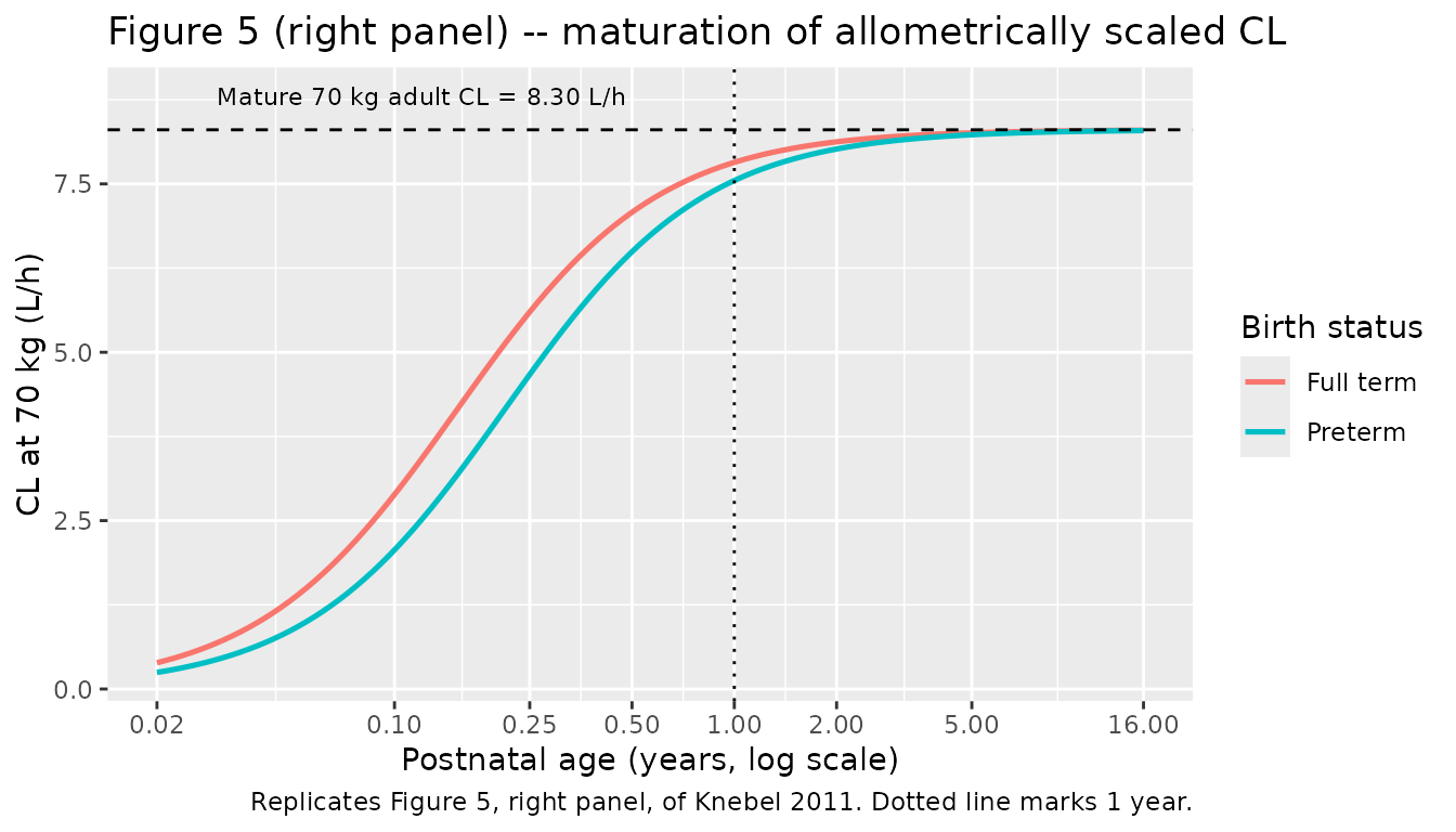
mat_at <- function(age, tb) {
  a50 <- 0.153 * 1.38^(1 - tb)
  age^1.48 / (age^1.48 + a50^1.48)
}
stopifnot(
  # "the age effect reached an asymptote approximately equal to the adult
  # allometrically scaled CL by 1" (Discussion): >= 90% of mature at 1 year for
  # both birth strata.
  mat_at(1, 1) > 0.90,
  mat_at(1, 0) > 0.90,
  # "Differences in allometrically scaled CL because of age are negligible,
  # after the age of 1 year" -- within 5% of mature from 2 years on.
  mat_at(2, 0) > 0.95,
  # Preterm infants are below full-term at every age before maturity.
  all(mat_at(age_grid, 0) < mat_at(age_grid, 1))
)
Figures 2 and 3: typical concentration-time profiles by formulation
Knebel 2011 Figures 2 and 3 present observed-versus-predicted and concentration-versus-time panels stratified by formulation. The observed data are not available, so the panel below shows the typical-value profile plus the 5th-95th percentile band from the simulated cohort, which is the model-side half of those figures.
sim |>
  filter(time <= tau) |>
  group_by(arm, time) |>
  summarise(Q05 = quantile(Cc, 0.05), Q50 = quantile(Cc, 0.50),
            Q95 = quantile(Cc, 0.95), .groups = "drop") |>
  ggplot(aes(time, Q50)) +
  geom_ribbon(aes(ymin = Q05, ymax = Q95), alpha = 0.25) +
  geom_line(linewidth = 0.8) +
  facet_wrap(~arm) +
  scale_y_log10() +
  labs(x = "Time after the first dose (h)", y = "Plasma pantoprazole (ng/mL)",
       title = "Simulated profiles by formulation, 1.2 mg/kg once daily",
       caption = "Model-side counterpart of Figures 2 and 3 of Knebel 2011. Median with 5th-95th percentile band.")
#> Warning in scale_y_log10(): log-10 transformation introduced infinite values.
#> log-10 transformation introduced infinite values.
#> log-10 transformation introduced infinite values.
#> log-10 transformation introduced infinite values.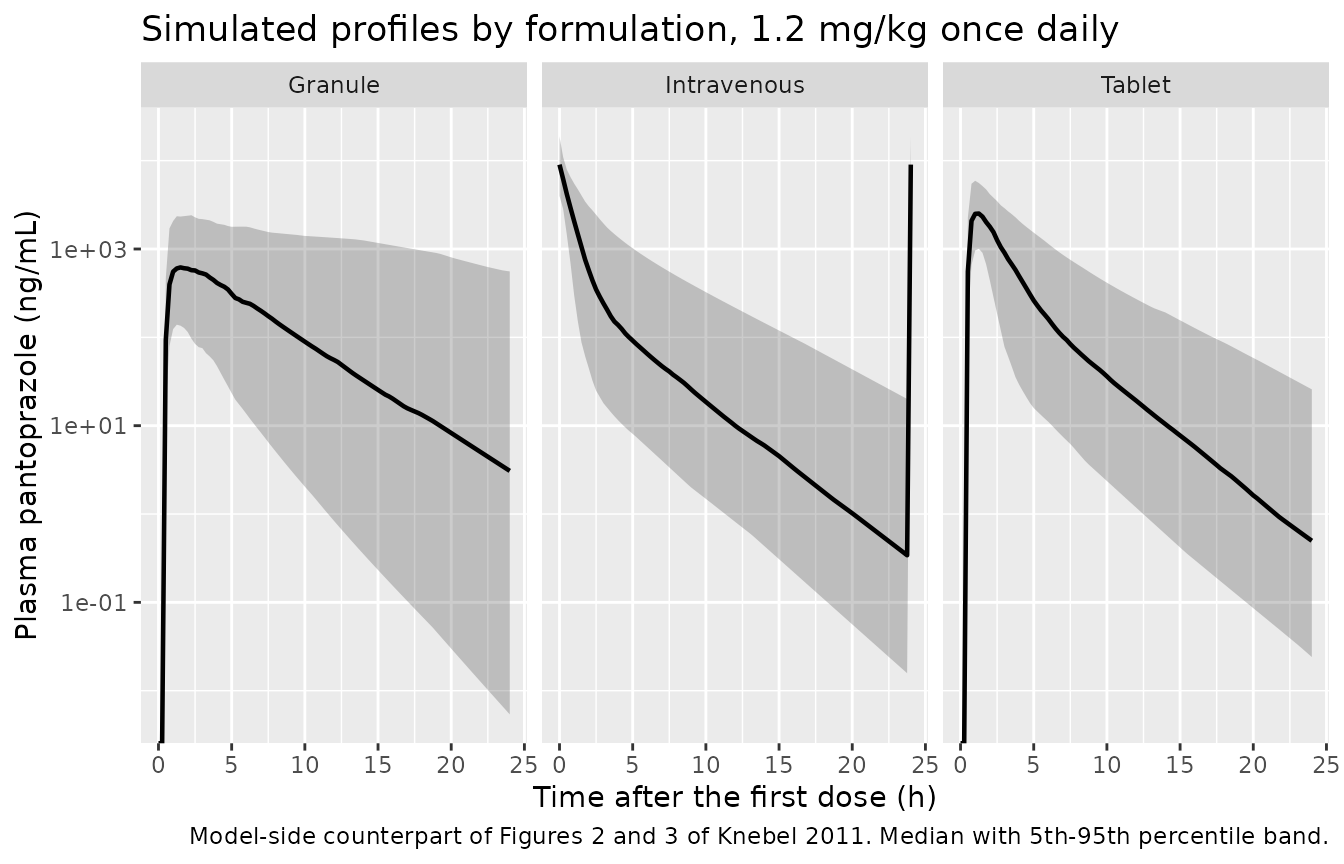
The tablet reaches a lower peak than the intravenous arm and the granule lower still, consistent with the published Ka and F1 estimates (tablet Ka 1.32 1/h and F1 fixed at 1; granule Ka 0.613 1/h and F1 0.295).
Figure 6: simulated AUCss by age bin for the 1.2 mg/kg scenario
Knebel 2011 Figure 6 (top right panel) shows simulated 24-hour
steady-state AUC for the 1.2 mg/kg scenario by age bin, against the
range of adult exposures after a 40 mg oral dose. The adult range itself
is drawn only as solid lines on the figure and is not tabulated anywhere
in the paper, so the reference line below is instead the adult
typical AUC implied by the model’s own 70 kg adult clearance
via equation 5 (AUCss = F * DOSE * 1000 / CL); the paper’s
minimum-to-maximum band would sit around it.
auc_by_subject <- sim |>
  filter(time >= t_last) |>
  group_by(id, arm) |>
  arrange(time, .by_group = TRUE) |>
  summarise(
    AUCss = sum(diff(time) * (head(Cc, -1) + tail(Cc, -1)) / 2),
    .groups = "drop"
  ) |>
  left_join(subjects |> select(id, AGE, WT), by = "id") |>
  mutate(age_bin = cut(AGE, breaks = c(0, 0.25, 0.5, 1, 2, 6, 16),
                       labels = c("<0.25", "0.25-0.5", "0.5-1", "1-2", "2-6", "6-16"),
                       include.lowest = TRUE))

adult_auc <- 40 * 1000 / adult_cl   # 40 mg oral, F = 1 (tablet anchor)

ggplot(auc_by_subject, aes(age_bin, AUCss)) +
  geom_boxplot(outlier.size = 0.6) +
  geom_hline(yintercept = adult_auc, linetype = "dashed", colour = "firebrick") +
  annotate("text", x = 0.7, y = adult_auc * 1.35, hjust = 0, colour = "firebrick",
           size = 3, label = sprintf("Adult 40 mg typical AUC = %.0f ng*h/mL", adult_auc)) +
  facet_wrap(~arm) +
  scale_y_log10() +
  labs(x = "Age bin (years)", y = "AUCss over 24 h (ng*h/mL)",
       title = "Figure 6 (scenario 1) -- steady-state AUC at 1.2 mg/kg by age bin",
       caption = "Replicates the 1.2-mg/kg panel of Figure 6 of Knebel 2011.")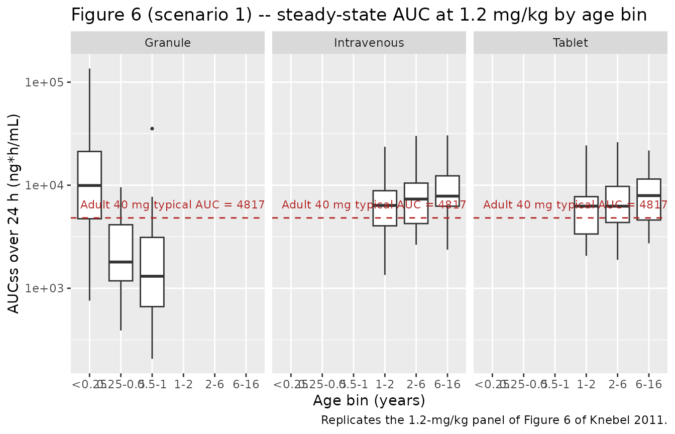
iv_tab_median <- auc_by_subject |>
  filter(arm %in% c("Intravenous", "Tablet")) |>
  group_by(age_bin) |>
  summarise(med = median(AUCss), .groups = "drop")

stopifnot(
  # Knebel 2011: scenario 1 "demonstrated distributions of AUCss that fell
  # within the adult AUC range for all age bins except 0.492 and 0.9 years".
  # The paper's adult range is figure-only, so the testable form of that claim
  # is that the F = 1 arms' bin medians sit within a factor of two of the adult
  # typical AUC across every bin -- a median-based check, not an extreme.
  # Guard: the check must actually have had bins to test. The two F = 1 arms
  # are the intravenous and tablet studies, which enrolled patients aged 1 to
  # 16 years, so they populate exactly the three bins from 1 year up; the three
  # infant bins belong to the granule arm and are dropped here by `group_by()`.
  identical(as.character(iv_tab_median$age_bin), c("1-2", "2-6", "6-16")),
  all(iv_tab_median$med > adult_auc / 2),
  all(iv_tab_median$med < adult_auc * 2)
)
PKNCA validation
Steady-state NCA over the final 24-hour dosing interval (144-168 h), stratified by formulation arm.
sim_nca <- sim |>
  filter(!is.na(Cc), time >= t_last) |>
  select(id, time, Cc, arm)

# Time-zero anchor for the interval: the concentration at 144 h is already the
# trough carried in from the previous dose, so no synthetic row is needed --
# but assert the interval start is present for every subject.
stopifnot(
  all(tapply(sim_nca$time, sim_nca$id, min) == t_last),
  nrow(sim_nca) > 0
)

conc_obj <- PKNCA::PKNCAconc(sim_nca, Cc ~ time | arm + id,
                             concu = "ng/mL", timeu = "h")

dose_df <- events |>
  filter(evid == 1L, time == t_last) |>
  select(id, time, amt, arm)

dose_obj <- PKNCA::PKNCAdose(dose_df, amt ~ time | arm + id, doseu = "mg")

intervals <- data.frame(
  start    = t_last,
  end      = t_last + tau,
  cmax     = TRUE,
  tmax     = TRUE,
  auclast  = TRUE,
  cav      = TRUE,
  half.life = TRUE
)

nca_res <- PKNCA::pk.nca(PKNCA::PKNCAdata(conc_obj, dose_obj, intervals = intervals))

nca_wide <- as.data.frame(nca_res) |>
  select(arm, id, PPTESTCD, PPORRES) |>
  tidyr::pivot_wider(names_from = PPTESTCD, values_from = PPORRES)

head(nca_wide) |>
knitr::kable(digits = 3, caption = "Per-subject steady-state NCA (first rows).")| arm | id | auclast | cmax | tmax | tlast | cav | lambda.z | r.squared | adj.r.squared | lambda.z.time.first | lambda.z.time.last | lambda.z.n.points | clast.pred | half.life | span.ratio |
|---|---|---|---|---|---|---|---|---|---|---|---|---|---|---|---|
| Granule | 301 | 2131.960 | 507.417 | 1.75 | 24 | 88.832 | 0.426 | 1 | 1 | 3.00 | 24 | 85 | 0.059 | 1.627 | 12.911 |
| Granule | 302 | 4753.742 | 436.553 | 2.75 | 24 | 198.073 | 0.102 | 1 | 1 | 6.00 | 24 | 73 | 51.966 | 6.799 | 2.647 |
| Granule | 303 | 6188.132 | 460.506 | 4.75 | 24 | 257.839 | 0.132 | 1 | 1 | 18.75 | 24 | 22 | 65.006 | 5.271 | 0.996 |
| Granule | 304 | 1218.727 | 418.784 | 1.50 | 24 | 50.780 | 0.322 | 1 | 1 | 9.25 | 24 | 60 | 0.071 | 2.152 | 6.854 |
| Granule | 305 | 13560.085 | 1804.985 | 2.25 | 24 | 565.004 | 0.170 | 1 | 1 | 7.25 | 24 | 68 | 46.933 | 4.078 | 4.107 |
| Granule | 306 | 1732.319 | 643.864 | 1.25 | 24 | 72.180 | 0.381 | 1 | 1 | 12.75 | 24 | 46 | 0.030 | 1.819 | 6.185 |
Comparison against the paper’s equation 5
Knebel 2011 does not publish an NCA table; the exposure metric it
does define analytically is equation 5,
AUCss_i = F * DOSE_i * 1000 / CL_i, which the authors used
to build Figure 6. Because equation 5 is exact for any linear model over
a full dosing interval at steady state, comparing PKNCA’s
auclast against it is a per-subject structural identity,
not a distributional comparison: both sides use the same drawn
parameters, so the only difference is trapezoidal error.
eq5 <- sim |>
  filter(time == t_last) |>
  distinct(id, arm, cl) |>
  left_join(dose_df |> select(id, amt), by = "id") |>
  mutate(
    f1     = if_else(arm == "Granule", 0.295, 1),
    AUC_eq5 = f1 * amt * 1000 / cl
  )

# The granule arm carries inter-occasion variability on F1, so its realised
# bioavailability is not the typical 0.295 and equation 5 with the typical F
# does not apply per subject. Restrict the identity to the arms with F = 1.
ident <- nca_wide |>
  left_join(eq5, by = c("id", "arm")) |>
  filter(arm != "Granule") |>
  mutate(pct_diff = 100 * (auclast / AUC_eq5 - 1))

tibble::tibble(
  Arm            = c("Intravenous", "Tablet"),
  `Median % difference` = vapply(c("Intravenous", "Tablet"),
    function(a) median(ident$pct_diff[ident$arm == a]), numeric(1)),
  `Max abs % difference` = vapply(c("Intravenous", "Tablet"),
    function(a) max(abs(ident$pct_diff[ident$arm == a])), numeric(1))
) |>
  knitr::kable(digits = 4,
caption = "PKNCA auclast over 144-168 h versus equation 5 (F * DOSE * 1000 / CL), per subject.")| Arm | Median % difference | Max abs % difference |
|---|---|---|
| Intravenous | 0.0648 | 0.3226 |
| Tablet | -0.0272 | 3.1012 |
stopifnot(
  # Both sides use the same drawn parameters, so the discrepancy is pure
  # trapezoidal error on the 0.25 h observation grid, not a distributional
  # difference. The median is therefore the structural check and is asserted
  # tightly: a mis-encoded F1, dose, or clearance would shift it by whole
  # percent, not by hundredths.
  abs(median(ident$pct_diff[ident$arm == "Intravenous"])) < 0.5,
  abs(median(ident$pct_diff[ident$arm == "Tablet"])) < 0.5,
  # Per-subject ceilings. The TABLET arm carries the larger error: its peak
  # falls in the middle of the interval, so PKNCA's lin-up/log-down rule spends
  # the whole absorption limb on the linear trapezoid, which overshoots a
  # convex rise. The intravenous profile peaks at the interval start, leaving
  # the window almost entirely log-down decay, where the rule is near-exact.
  # Measured maxima are 3.1% (tablet) and 0.32% (intravenous); the bounds below
  # leave room for which ka/kel pairs a given rxode2 build happens to draw.
  all(abs(ident$pct_diff[ident$arm == "Tablet"]) < 6.0),
  all(abs(ident$pct_diff[ident$arm == "Intravenous"]) < 1.5)
)
The granule arm is excluded above because its realised F1 carries the inter-occasion random effect. Its typical exposure ratio is still an exact consequence of the published F1, and is checked deterministically:
# One matched pair of typical subjects differing only in formulation.
pair <- bind_rows(
  subjects |> filter(arm == "Tablet")  |> slice(1) |> mutate(id = 1L),
  subjects |> filter(arm == "Tablet")  |> slice(1) |>
    mutate(id = 2L, arm = "Granule", FORM_TABLET = 0L, FORM_GRANULE = 1L)
)
pair_ev <- bind_rows(
  pair |> tidyr::crossing(dose_no = seq_len(n_dose)) |>
    mutate(time = (dose_no - 1) * tau, amt = 1.2 * WT, evid = 1L, cmt = "depot",
           OCC = if_else(dose_no == 1L, 1L, 2L)) |> select(-dose_no),
  pair |> tidyr::crossing(time = seq(t_last, t_last + tau, by = 0.05)) |>
    mutate(amt = NA_real_, evid = 0L, cmt = "central", OCC = 2L)
) |> arrange(id, time, desc(evid))

pair_sim <- as.data.frame(rxode2::rxSolve(mod0, pair_ev, returnType = "data.frame"))
#> ℹ omega/sigma items treated as zero: 'etalcl', 'etalvc', 'etalka', 'etaiov_fdepot_1', 'etaiov_fdepot_2'
#> Warning: multi-subject simulation without without 'omega'
pair_auc <- pair_sim |>
  group_by(id) |>
  arrange(time, .by_group = TRUE) |>
  summarise(AUC = sum(diff(time) * (head(Cc, -1) + tail(Cc, -1)) / 2), .groups = "drop")

granule_ratio <- pair_auc$AUC[pair_auc$id == 2L] / pair_auc$AUC[pair_auc$id == 1L]
cat(sprintf("Granule / tablet steady-state AUC ratio: %.5f (published F1 spheroid = 0.295)\n",
            granule_ratio))
#> Granule / tablet steady-state AUC ratio: 0.29502 (published F1 spheroid = 0.295)

stopifnot(abs(granule_ratio - 0.295) < 1e-4)
Simulated NCA summary versus the equation-5 reference
reference <- eq5 |>
  filter(arm != "Granule") |>
  group_by(arm) |>
  summarise(auclast = median(AUC_eq5), .groups = "drop")

cmp <- nlmixr2lib::ncaComparisonTable(
  simulated     = nca_res,
  reference     = reference,
  by            = "arm",
  units         = c(auclast = "ng*h/mL"),
  tolerance_pct = 20
)

knitr::kable(
  cmp,
  caption = "Simulated steady-state AUC0-tau versus the equation-5 reference (median across subjects). * marks a difference above 20%.",
  align   = c("l", "l", "r", "r", "r")
)| NCA parameter | arm | Reference | Simulated | % diff |
|---|---|---|---|---|
| AUClast (ng*h/mL) | Intravenous | 7050 | 7060 | +0.1% |
| AUClast (ng*h/mL) | Tablet | 6720 | 6720 | -0.0% |
Assumptions and deviations
-
Equation 6 is a NONMEM
$PKdefault-then-override block. The printed equation setsKa = theta5,ALAG1 = theta6, andF1_tablet = theta7, then opens anIf (spheroid)branch that overridesKaandF1only. The lag time is therefore applied to both oral formulations. Table IV supports this: the “Ka” and “F1” rows are explicitly labelled per formulation (“Ka tablet”, “Ka spheroid”, “F1 tablet”, “F1 spheroid”) while the “Lag Time (hour)” row carries no formulation label. -
Three formulations, two indicator columns. The
{intravenous, tablet, granule}stratification is encoded asFORM_TABLET+FORM_GRANULEwith both zero selecting the intravenous route. This is the three-level construction already used byKleideiter_2017_cebranopadolandWada_2023_sparsentan; note that the reference category for both indicators here is the intravenous route rather than the oral-liquid or tablet comparators named as the defaults in the covariate register. -
The sex effect is applied to
(1 - SEXF). Knebel 2011 codes sex as 0 = female / 1 = male and names female as a reference covariate, so the published 1.06 is the male multiplier. The canonical column isSEXF(1 = female), so the coefficient is raised to(1 - SEXF)to keep the published number verbatim. -
TERM_BIRTHuses the paper’s 38-week cutoff. Knebel 2011 defines preterm as gestational age below 38 weeks, not the 37-week obstetric convention named in the canonical register entry. Assemble the column with the paper’s rule when driving this model. -
Emaxis written as the literal 1 in the maturation sigmoid, because the paper fixed it structurally (“The maximum effect (Emax) was fixed at 1”) and Table IV reports no Emax row. It is not anini()parameter. -
Inter-occasion variability is expanded into two
occasion-indexed etas. Equation 6 writes
F1_spheroid = theta8 * exp(eta_OCC1 + eta_OCC2), the NONMEM idiom where exactly one eta is active per occasion and both share one variance. rxode2 cannot simulate theeta ~ var | OCCform, so the model uses theoc1/oc2multiplexed expansion (as inChen_2023_nemonoxacinandJonsson_2011_ethambutol), with the second variance fixed to the first. This emits a benignsome etas defaulted to non-mu referencedwarning at load; it affects estimation only, not simulation. -
Concentration units are ng/mL, matching the assay.
Amounts are in mg and volumes in L, so
Cccarries an explicit factor of 1000. The additive residual SD of 6.08 ng/mL only makes sense on this scale (the assay LLOQ was 10 ng/mL). - Below-quantification data were excluded by the authors, not modelled with an M3-type likelihood, so the model has no BLQ handling.
-
The intravenous arm is simulated as a bolus. Knebel
2011 gives the intravenous doses (0.8 or 1.6 mg/kg) but never states an
infusion duration, and the model file carries no infusion term –
administration duration is a property of the event table, not of the
model, so a user with the real infusion times can supply
rateorduron the dose records without touching the model. The choice does not affect any assertion here: steady-state AUC over a full dosing interval isF * Dose / CLfor any infusion duration, so only the simulated intravenous Cmax (not AUC) would change. - Virtual-cohort weight is drawn from a WHO / CDC median weight-for-age curve with 20% lognormal scatter. Knebel 2011 reports only marginal weight and age summaries (Table I), never their joint distribution, so a weight-for-age relationship had to be assumed. The resulting pooled cohort median weight is compared against Table I in the cohort chunk.
-
The simulated cohort carries no CYP2C19 poor
metabolizers. Knebel 2011 presents its simulation results “only
for extensive metabolizers … because of the limited number of poor
metabolizers” (n = 4), and the model file’s
CYP2C19_PMeffect is validated separately in the answer-key table above. - Preterm status is assigned only in the infant arm. Table I records gestational age for the 119 patients aged birth to 11 months; the 1-to-16-year arms are treated as full term.
- The adult reference AUC in the Figure 6 replication is model-derived, not transcribed. The paper’s adult 40 mg exposure range comes from an unpublished NDA submission (“data on file at Wyeth”) and appears only as solid lines on Figure 6, with no numeric values anywhere in the text. The replication therefore uses the adult typical AUC implied by the model’s own 70 kg clearance through equation 5, and the assertion is framed on bin medians within a factor of two rather than on the paper’s un-transcribed band.
- No parameter value in this model came from anywhere other than Knebel 2011’s own text and Table IV. No author correspondence, figure digitisation, or upstream-model transfer was required.
Errata and source-quality notes
The Discussion’s IOV interval disagrees with Table IV
The Discussion reports the granule bioavailability inter-occasion variability as “a point estimate (95% CI) interoccasion CV of 56.7% (37.7, 61.4)”. Table IV’s OMEGA4.4 row gives the variance as 0.321 with a bootstrap 95% CI of (0.142, 0.519). Taking square roots:
tibble::tibble(
  Quantity    = c("Point estimate", "Lower 95% bound", "Upper 95% bound"),
  `Table IV variance` = c(0.321, 0.142, 0.519),
  `sqrt(variance), %` = round(100 * sqrt(c(0.321, 0.142, 0.519)), 1),
  `Discussion, %`     = c(56.7, 37.7, 61.4)
) |>
knitr::kable(caption = "The Discussion's IOV point estimate and lower bound reproduce Table IV exactly under the square-root rule; its upper bound does not.")| Quantity | Table IV variance | sqrt(variance), % | Discussion, % |
|---|---|---|---|
| Point estimate | 0.321 | 56.7 | 56.7 |
| Lower 95% bound | 0.142 | 37.7 | 37.7 |
| Upper 95% bound | 0.519 | 72.0 | 61.4 |
The point estimate (56.7) and the lower bound (37.7) reproduce Table
IV exactly as the square root of the printed variance, so the
upper bound should be 72.0%, not 61.4%. This cuts two ways. It is a
genuine internal inconsistency in the paper – but because two of the
three numbers match to the last printed digit, it is also independent
corroboration of this vignette’s central decoding decision above: Table
IV’s “CV%” column really is the plain square root of the printed
variance, not a log-normal sqrt(exp(omega^2) - 1)
transform. The model uses only the point estimate, so nothing downstream
depends on which bound is right.
Table I labelling and internal consistency
Three further labelling or consistency problems, all in Table I. None
affects the model, since none of the affected rows feeds a parameter –
AGE is a data column the user supplies, not an
estimate.
- The row “Preterm age, mos” reports a minimum of 1, maximum of 15, and median of 6. The Results text describes the same 77 patients as “ranging from 1 to 15 weeks preterm”, so the column header’s unit (“mos”) contradicts the paper’s own prose; the values are weeks preterm.
- The row “Corrected age,” has no unit in the header at all. Its values (33.3 to 43.7, median 37.5, n = 50) are consistent with postmenstrual age in weeks.
- The two age rows contradict each other – Table I carries both “Age, y” and “Age, wks” for the same N = 202, but neither is a unit conversion of the other. See the table below.
| Statistic | Age, y (Table I) | Implied weeks | Age, wks (Table I) |
|---|---|---|---|
| Minimum | 0.025 | 1.3 | 0.3 |
| Maximum | 16.000 | 834.8 | 192.0 |
| Median | 0.650 | 33.9 | 7.8 |
| Mean | 3.690 | 192.5 | 44.3 |
Sixteen years is 835 weeks, not 192, and 0.65 years is 33.9 weeks, not 7.8. Only the years row is consistent with the paper’s own title and abstract (“birth to 16 years”) and with the 1-to-16-year intravenous and tablet arms, so this vignette quotes and simulates the years row throughout. (The “Age, wks” maximum of 192 weeks equals 3.68 years, which is numerically the mean of the years row – suggestive of a transcription slip in that row, though the paper gives no way to confirm it.)