Tramadol (Soria-Chacartegui 2026)
Source:vignettes/articles/SoriaChacartegui_2026_tramadol.Rmd
SoriaChacartegui_2026_tramadol.RmdModel and source
- Citation: Soria-Chacartegui P, Wurthwein G, Zubiaur P, Almenara S, Ochoa D, Abad-Santos F, Hempel G. Role of Pharmacogenetics on Tramadol Pharmacokinetics: A Population Pharmacokinetic Model. Eur J Drug Metab Pharmacokinet. 2026;51(2):205-216. doi:10.1007/s13318-026-00986-3.
- Description: Two-compartment population PK model for oral tramadol in European healthy volunteers (Soria-Chacartegui 2026), with a Savic transit-compartment chain delivering the dose into a depot compartment, first-order absorption from the depot into the central compartment, first-order elimination, a linear body-weight effect on the central volume, and a CYP2D6 intermediate-metabolizer effect that lowers clearance by 19.8% relative to the pooled normal-plus-ultrarapid-metabolizer reference group.
- Article: https://doi.org/10.1007/s13318-026-00986-3
- Supplement (open access, includes the differential equations as Figure S1 and the structural model-building table S2): https://doi.org/10.1007/s13318-026-00986-3
Population
Soria-Chacartegui 2026 fitted 24 European healthy volunteers (17 men, 7 women) enrolled in a phase I, open-label, randomized, replicated crossover bioequivalence trial (EUDRA-CT 2013-000196-32) at the Hospital Universitario de La Princesa, Madrid. Only the reference arm was modelled: a single oral dose of 37.5 mg tramadol hydrochloride oral drops (Adolonta) co-administered with 400 mg ibuprofen arginine oral solution (Espidifen), under fasting conditions.
Median age was 24 years (IQR 22 to 27), median height 1.72 m (IQR 1.67 to 1.77), median weight 70.0 kg (IQR 66.2 to 74.2) and median BMI 22.6 kg/m2 (IQR 21.8 to 25.5); trial eligibility required a BMI between 18.5 and 30 kg/m2 (Table 1). Women were significantly shorter and lighter than men (both p < 0.001). Each volunteer contributed a pre-dose baseline sample plus 18 post-dose plasma samples from 0.25 h to 24 h, assayed by LC-MS/MS over a 0.5 to 250 ng/mL calibration range; every post-dose sample was above the 0.5 ng/mL LLOQ (Supplementary Material).
Volunteers were genotyped for 180 variants (Supplementary Table S1) and CYP2D6, CYP2B6 and CYP3A4 phenotypes were inferred per CPIC and DPWG. The CYP2D6 split was 8 intermediate metabolizers (IMs), 14 normal metabolizers (NMs) and 2 ultrarapid metabolizers (UMs), with no poor metabolizers; NMs and UMs were pooled to gain power (Methods 2.4).
The same information is available programmatically via
readModelDb("SoriaChacartegui_2026_tramadol")()$population.
Source trace
Every ini() entry in
inst/modeldb/specificDrugs/SoriaChacartegui_2026_tramadol.R
carries an in-file comment naming its origin. They are collected here
for review.
| Equation / parameter | Value | Source location |
|---|---|---|
lcl (CL/F) |
51.1 L/h | Table 2, row “CL (L/h)”; RSE 6.5%, bootstrap 51.3 (44.8 to 58.3) |
lvc (Vc/F at 70 kg) |
126 L | Table 2, row “Vc (L)”; RSE 14.3%, bootstrap 127 (84.0 to 173) |
lq (Q/F) |
175 L/h | Table 2, row “Q (L/h)”; RSE 14.3%, bootstrap 171 (133 to 232) |
lvp (Vp/F) |
171 L | Table 2, row “Vp (L)”; RSE 8.2%, bootstrap 169 (141 to 204) |
lka (Ka) |
3.09 1/h | Table 2, row “Ka (h-1)”; RSE 20%, bootstrap 3.15 (2.07 to 5.01) |
lmtt (MTT) |
0.24 h | Table 2, row “MTT (h)”; RSE 5.4%, bootstrap 0.24 (0.21 to 0.27) |
lntr (NCMT) |
17.6 | Table 2, row “NCMT”; RSE 18.7%, bootstrap 17.5 (11.3 to 90.1) |
e_cyp2d6_im_cl |
-0.198 | Table 2, row “Being CYP2D6 IM as covariate for CL”; Results 3.2 states the 19.8% CL reduction |
e_wt_vc |
0.0311 per kg | Table 2, row “Weight as covariate for Vc”; RSE 31.3%, bootstrap 0.0303 (0.0081 to 0.0486) |
etalcl variance |
0.088949 | Table 2, “IIV CL (%)” = 30.5, back-transformed by footnote (3) |
etalvc variance |
0.383803 | Table 2, “IIV Vc (%)” = 68.4, back-transformed by footnote (3) |
etalka variance |
0.773067 | Table 2, “IIV Ka (%)” = 108, back-transformed by footnote (3) |
etalmtt variance |
0.041956 | Table 2, “IIV MTT (%)” = 20.7, back-transformed by footnote (3) |
etalcl / etalvc covariance |
not reported | Table 2 footnote (2) and Results 3.2 state an OMEGA block exists; no value is published (see Assumptions) |
propSd |
0.0983 | Table 2, “Proportional residual error” = 9.83%; RSE 5.5%, bootstrap 9.60 (8.60 to 10.8) |
addSd |
fixed 0.01 ng/mL | Table 2 footnote (1); Results 3.2 gives the units |
| Transit chain, depot, central and peripheral ODEs | n/a | Supplementary Figure S1 (reproduced in the model file header comments); Figure 2 schematic |
ktr = (ntr + 1) / mtt |
n/a | Derived from Supplementary Figure S1 (see below) |
| Weight centring value 70 kg | n/a | Table 1 “Total” row median weight; Methods 2.4 simulations run at weight = 70 kg |
Why ktr = (ntr + 1) / mtt
Supplementary Figure S1 writes the absorption chain as
dA_0/dt   = Dose input - Ktr * A_0
dA_i/dt   = Ktr * A_(i-1) - Ktr * A_i,   i = 1..n
dA_dep/dt = Ktr * A_n - Ka * A_dep
so a dose molecule crosses n + 1 first-order steps of
rate Ktr between the dose record and the depot. Its arrival
time in the depot is therefore Erlang-distributed with shape
n + 1 and mean (n + 1) / Ktr, and that mean is
what the paper reports as MTT. This is the Savic 2007 convention, the
same one rxode2::transit() uses. At the typical values,
ktr = 18.6 / 0.24 = 77.5 1/h.
Because NCMT is estimated as a real number (17.6), the chain cannot be written as an integer number of ODE states; the model file evaluates the gamma density the chain converges to, which is exactly what NONMEM fits in this situation.
Virtual cohort
The original data are not publicly available (Data Availability Statement). The cohort below reproduces the paper’s own simulation setup in Methods 2.4: model individuals fixed at weight = 70 kg, stratified by CYP2D6 phenotype, under a single 37.5 mg dose and at steady state with an 8 h dosing interval. The paper used 1000 individuals per stratum; 200 per arm is used here (the nlmixr2lib cohort cap), which is ample for the median and 2.5th/97.5th percentile summaries reported in Table 4 and Figure 5.
dose_mg <- 37.5
tau <- 8

# Steady state is approached at the terminal rate; with a terminal half-life of
# ~4.4 h (NM+UM) to ~5.4 h (IM), 11 priming doses at 8 h intervals put the
# system more than 10 terminal half-lives in, so the 12th dose at t = 88 h is
# given at steady state. The paper's NONMEM SS = 1 / II = 8 record with a single
# dose row means the profile after that dose has NO further doses, which is what
# the observation window 88 to 112 h reproduces here.
ss_last_dose <- 88
ss_dose_times <- seq(0, ss_last_dose, by = tau)

# Post-dose grid: dense through the absorption pulse (MTT = 0.24 h, chain SD
# ~0.056 h), coarser through the terminal phase. A grid that cannot resolve Tmax
# understates AUC and Cmax, so the absorption window is sampled at 0.01 h.
post_dose_grid <- sort(unique(c(
  seq(0, 1.5, by = 0.01),
  seq(1.5, 4, by = 0.05),
  seq(4, 24, by = 0.25)
)))

# Priming intervals only need enough observation times to stop the ODE solver
# from stepping over each narrow absorption pulse.
prime_grid <- sort(unique(as.vector(outer(
  seq(0, ss_last_dose - tau, by = tau),
  c(0.05, 0.1, 0.15, 0.2, 0.25, 0.3, 0.4, 0.6, 1, 2, 4, 6),
  "+"
))))

make_arm <- function(n, cyp2d6_im, dose_times, obs_times, arm, id_offset) {
  subj <- tibble(
    id = id_offset + seq_len(n),
    WT = 70,
    CYP2D6_IM = cyp2d6_im,
    arm = arm
  )
  bind_rows(
    expand_grid(subj, time = dose_times) |>
      mutate(evid = 1L, amt = dose_mg, cmt = "depot"),
    # cmt is the ODE STATE name; rxode2 returns the algebraic observable Cc as
    # a column at these rows automatically.
    expand_grid(subj, time = obs_times) |>
      mutate(evid = 0L, amt = NA_real_, cmt = "central")
  ) |>
    arrange(id, time, desc(evid))
}

n_per_arm <- 200L

ev_sd_nm <- make_arm(n_per_arm, 0, 0, post_dose_grid,
                     "NM+UM, single dose", 0L)
ev_sd_im <- make_arm(n_per_arm, 1, 0, post_dose_grid,
                     "IM, single dose", 1000L)
ev_ss_nm <- make_arm(n_per_arm, 0, ss_dose_times,
                     sort(unique(c(prime_grid, ss_last_dose + post_dose_grid))),
                     "NM+UM, steady state", 2000L)
ev_ss_im <- make_arm(n_per_arm, 1, ss_dose_times,
                     sort(unique(c(prime_grid, ss_last_dose + post_dose_grid))),
                     "IM, steady state", 3000L)

events <- bind_rows(ev_sd_nm, ev_sd_im, ev_ss_nm, ev_ss_im)
stopifnot(!anyDuplicated(unique(events[, c("id", "time", "evid")])))
Simulation
Each arm is solved in its own rxSolve() call, reseeded
to the same value immediately beforehand. That gives the IM and NM+UM
arms common random numbers: subject i
draws the same etalcl, etalvc,
etalka and etalmtt in both phenotypes, so the
phenotype contrast is the covariate effect alone and not Monte-Carlo
noise. This turns the published IM-versus-NM exposure ratio into an
exact gate rather than a noisy one.
mod <- readModelDb("SoriaChacartegui_2026_tramadol")

solve_arm <- function(ev) {
  rxode2::rxSetSeed(20260303)
  rxode2::rxSolve(
    mod,
    events = ev,
    keep = c("WT", "CYP2D6_IM", "arm"),
    returnType = "data.frame"
  )
}

sim <- bind_rows(lapply(
  list(ev_sd_nm, ev_sd_im, ev_ss_nm, ev_ss_im),
  solve_arm
))
#> ℹ parameter labels from comments will be replaced by 'label()'

# rxSolve returns every quantity computed inside model(), including the
# individual clearance, which Table 4 reports directly (see the NCA section).
stopifnot(all(c("Cc", "cl", "vc") %in% names(sim)))
stopifnot(!anyNA(sim$Cc))
sim$arm <- factor(sim$arm, levels = c(
  "NM+UM, single dose", "IM, single dose",
  "NM+UM, steady state", "IM, steady state"
))
Structural checks
These three checks compare the packaged model against closed-form consequences of the published parameters. Both sides of each comparison use the same drawn parameters, so the residual is pure numerical error and the tolerances are tight; they are regression gates, not distributional claims.
theta <- rxode2::rxode(mod)$theta
#> ℹ parameter labels from comments will be replaced by 'label()'
cl_typ <- exp(theta[["lcl"]])
vc_typ <- exp(theta[["lvc"]])
q_typ <- exp(theta[["lq"]])
vp_typ <- exp(theta[["lvp"]])

# --- 1. Mass balance: the whole 37.5 mg dose must reach the systemic
# circulation. The transit chain is evaluated in closed form from podo()/tad()
# with the depot bolus suppressed by f(depot) <- 0, so a sign or gamma-shape
# error would silently deliver the wrong amount. AUC(0, Inf) * CL == Dose is the
# exact identity that detects it.
typ_grid <- sort(unique(c(seq(0, 2, by = 0.002), seq(2, 240, by = 0.05))))
ev_typ <- bind_rows(
  tibble(id = 1L, time = 0, evid = 1L, amt = dose_mg, cmt = "depot"),
  tibble(id = 1L, time = typ_grid, evid = 0L, amt = NA_real_, cmt = "central")
) |>
  mutate(WT = 70, CYP2D6_IM = 0) |>
  arrange(time, desc(evid))

sim_typ <- rxode2::rxSolve(rxode2::zeroRe(mod), ev_typ,
                           returnType = "data.frame")
#> ℹ parameter labels from comments will be replaced by 'label()'
#> ℹ omega/sigma items treated as zero: 'etalcl', 'etalvc', 'etalka', 'etalmtt'
obs_typ <- sim_typ[!is.na(sim_typ$Cc), ]
auc_typ <- sum(diff(obs_typ$time) *
                 (head(obs_typ$Cc, -1) + tail(obs_typ$Cc, -1)) / 2)
# Cc is ng/mL and dose is mg, so AUC (ng*h/mL) * CL (L/h) is in ug: 37.5 mg dose
# corresponds to 37500 ug.
delivered_ug <- auc_typ * cl_typ
mass_balance_err <- delivered_ug / (dose_mg * 1000) - 1

# --- 2. Terminal half-life against the analytic beta of the 2-compartment
# system built from the published CL, Vc, Q and Vp.
analytic_beta <- function(cl, vc, q, vp) {
  kel <- cl / vc
  k23 <- q / vc
  k32 <- q / vp
  s <- kel + k23 + k32
  (s - sqrt(s^2 - 4 * kel * k32)) / 2
}
beta_nm <- analytic_beta(cl_typ, vc_typ, q_typ, vp_typ)
# Keep Cc >= 1e-6 of Cmax: below that the ODE tail is solver noise.
tail_typ <- obs_typ[obs_typ$time > 48 & obs_typ$time < 200 &
                      obs_typ$Cc >= 1e-6 * max(obs_typ$Cc), ]
beta_sim <- -coef(lm(log(Cc) ~ time, tail_typ))[[2]]

# --- 3. Steady-state volume. The Discussion reports Vd = 297 L, which is
# exactly Vc + Vp at the 70 kg centring weight; this pins the centring value.
vss_typ <- vc_typ + vp_typ

structural <- tibble(
  Check = c(
    "Dose delivered through the transit chain (fraction of 37.5 mg)",
    "Terminal half-life, simulated (h)",
    "Terminal half-life, analytic beta (h)",
    "Vc + Vp at 70 kg (L)"
  ),
  Simulated = c(1 + mass_balance_err, log(2) / beta_sim,
                log(2) / beta_nm, vss_typ),
  Expected = c(1, log(2) / beta_nm, log(2) / beta_nm, 297),
  Source = c(
    "mass balance: AUC(0,Inf) * CL = Dose",
    "closed form from Table 2 CL/Vc/Q/Vp",
    "closed form from Table 2 CL/Vc/Q/Vp",
    "Discussion: 'the reported volume of distribution (Vd) (297 L)'"
  )
)
knitr::kable(structural, digits = 4,
caption = "Structural consistency of the packaged model.")| Check | Simulated | Expected | Source |
|---|---|---|---|
| Dose delivered through the transit chain (fraction of 37.5 mg) | 1.0000 | 1.0000 | mass balance: AUC(0,Inf) * CL = Dose |
| Terminal half-life, simulated (h) | 4.4456 | 4.4456 | closed form from Table 2 CL/Vc/Q/Vp |
| Terminal half-life, analytic beta (h) | 4.4456 | 4.4456 | closed form from Table 2 CL/Vc/Q/Vp |
| Vc + Vp at 70 kg (L) | 297.0000 | 297.0000 | Discussion: ‘the reported volume of distribution (Vd) (297 L)’ |
stopifnot(
  # The transit chain must deliver the entire dose.
  abs(mass_balance_err) < 0.005,
  # The simulated terminal slope must match the closed form.
  abs(log(2) / beta_sim - log(2) / beta_nm) < 0.02,
  # Vc + Vp must reproduce the Discussion's 297 L, which is what fixes the
  # weight-centring value at 70 kg.
  abs(vss_typ - 297) < 0.5
)
The typical-value terminal half-life is 4.45 h, matching the 4.5 h the paper reports in Table 3 and quotes in the Discussion.
Replicate published figures
# Replicates Figure 5 of Soria-Chacartegui 2026: simulated concentration-time
# curves for 37.5 mg tramadol as (A) a single oral dose and (B) a dose at steady
# state with an 8 h dosing interval, stratified by CYP2D6 phenotype. The bold
# line is the median and the shaded band the 2.5th to 97.5th percentile
# prediction interval, as in the published figure.
fig5 <- sim |>
  mutate(
    panel = if_else(grepl("single dose", arm),
                    "A: 37.5 mg single dose",
                    "B: 37.5 mg dose at steady state"),
    phenotype = if_else(grepl("^IM", arm),
                        "CYP2D6 IM", "CYP2D6 NM + UM"),
    tad_h = if_else(grepl("single dose", arm), time, time - ss_last_dose)
  ) |>
  filter(tad_h >= 0) |>
  group_by(panel, phenotype, tad_h) |>
  summarise(
    Q025 = quantile(Cc, 0.025),
    Q50 = quantile(Cc, 0.50),
    Q975 = quantile(Cc, 0.975),
    .groups = "drop"
  )

ggplot(fig5, aes(tad_h, Q50, colour = phenotype, fill = phenotype)) +
  geom_ribbon(aes(ymin = Q025, ymax = Q975), alpha = 0.20, colour = NA) +
  geom_line(linewidth = 0.8) +
  facet_wrap(~panel) +
  scale_colour_manual(values = c("CYP2D6 NM + UM" = "#c0392b",
                                 "CYP2D6 IM" = "#2c5f9e")) +
  scale_fill_manual(values = c("CYP2D6 NM + UM" = "#c0392b",
                               "CYP2D6 IM" = "#2c5f9e")) +
  labs(
    x = "Time after dose (h)", y = "Tramadol plasma concentration (ng/mL)",
    colour = NULL, fill = NULL,
    title = "Figure 5 - simulated profiles by CYP2D6 phenotype",
    caption = "Replicates Figure 5 of Soria-Chacartegui 2026."
  ) +
  theme(legend.position = "bottom")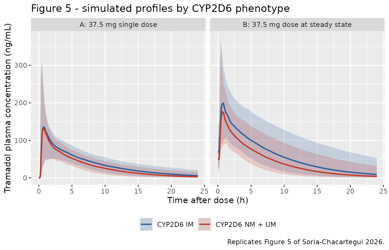
The paper’s Figure 4 is a VPC against the observed data, which are not public, so it cannot be replicated here. Figure 3 (goodness-of-fit) likewise requires the observed concentrations.
PKNCA validation
Each arm is reduced to a single dose followed by an observation
window, which is exactly the paper’s simulation design: for the
steady-state arms the NONMEM SS = 1 / II = 8
record with one dose row means no further doses follow, so the window 88
to 112 h is shifted to start at time 0 and its time-zero concentration
is the steady-state trough (not zero).
sim_nca <- sim |>
  filter(!is.na(Cc)) |>
  mutate(time = if_else(grepl("steady state", arm),
                        time - ss_last_dose, time)) |>
  filter(time >= 0) |>
  # Per subject, keep Cc >= 1e-6 of Cmax after the peak: below that the ODE tail is solver noise.
  group_by(arm, id) |>
  filter(time <= time[which.max(Cc)] | Cc >= 1e-6 * max(Cc)) |>
  ungroup() |>
  select(id, time, Cc, arm)

# Fail loudly if any subject lost its time-zero anchor; PKNCA would otherwise
# warn per subject and silently start AUC at the first available sample.
t0_count <- sim_nca |> filter(time == 0) |> distinct(id) |> nrow()
stopifnot(t0_count == 4L * n_per_arm)

dose_df <- events |>
  filter(evid == 1L) |>
  mutate(time = if_else(grepl("steady state", arm),
                        time - ss_last_dose, time)) |>
  filter(time == 0) |>
  select(id, time, amt, arm)
stopifnot(nrow(dose_df) == 4L * n_per_arm)

conc_obj <- PKNCA::PKNCAconc(sim_nca, Cc ~ time | arm + id)
dose_obj <- PKNCA::PKNCAdose(dose_df, amt ~ time | arm + id)

intervals <- data.frame(
  start = 0,
  end = Inf,
  cmax = TRUE,
  tmax = TRUE,
  auclast = TRUE,
  aucinf.obs = TRUE,
  half.life = TRUE,
  lambda.z = TRUE
)

nca_res <- PKNCA::pk.nca(PKNCA::PKNCAdata(conc_obj, dose_obj,
                                          intervals = intervals))
Comparison against published NCA
Table 4 of Soria-Chacartegui 2026 reports geometric means (and median
for Tmax) over their 1000 simulated individuals. For a log-normal
quantity the geometric mean equals the median, which is the summary
ncaComparisonTable() computes, so the two are directly
comparable.
Two of the seven rows are not NCA-derived in the
source. Table 4’s CL is the individual model clearance, not
Dose / AUCinf: for the steady-state NM + UM arm
Dose / AUCinf is 37500 / 1060 = 35.4 L/h,
which is nowhere near the tabulated 50.9 L/h, whereas the model’s
typical CL is 51.1 L/h. Vd is correspondingly
CL / lambda_z (for that arm,
50.9 / (log(2) / 4.2) = 308 L, the tabulated value). Both
are therefore reconstructed the same way here.
nca_wide <- as.data.frame(nca_res$result) |>
  filter(PPTESTCD %in% c("cmax", "tmax", "auclast",
                         "aucinf.obs", "half.life", "lambda.z")) |>
  select(arm, id, PPTESTCD, PPORRES) |>
  pivot_wider(names_from = PPTESTCD, values_from = PPORRES)

# Individual model clearance, one value per subject (constant over time).
cl_ind <- sim |>
  group_by(arm, id) |>
  summarise(cl = first(cl), .groups = "drop")

simulated <- nca_wide |>
  left_join(cl_ind, by = c("arm", "id")) |>
  mutate(
    cl.obs = cl,             # Table 4 "CL": the individual model clearance
    vz.obs = cl / lambda.z   # Table 4 "Vd": CL / lambda_z
  ) |>
  group_by(arm) |>
  summarise(across(c(cmax, tmax, auclast, aucinf.obs,
                     half.life, cl.obs, vz.obs), median),
            .groups = "drop") |>
  mutate(arm = as.character(arm))

published <- tibble::tribble(
  ~arm,                   ~cmax, ~tmax, ~auclast, ~aucinf.obs, ~half.life, ~cl.obs, ~vz.obs,
  "NM+UM, single dose",     139,  0.71,      717,         739,        4.2,    51.0,     309,
  "IM, single dose",        140,  0.75,      859,         911,        5.3,    41.3,     316,
  "NM+UM, steady state",    185,  0.70,     1030,        1060,        4.2,    50.9,     308,
  "IM, steady state",       203,  0.73,     1390,        1480,        5.3,    40.9,     311
)

cmp <- nlmixr2lib::ncaComparisonTable(
  simulated = simulated,
  reference = published,
  by = "arm",
  units = c(cmax = "ng/mL", tmax = "h", auclast = "ng*h/mL",
            aucinf.obs = "ng*h/mL", half.life = "h",
            cl.obs = "L/h", vz.obs = "L"),
  tolerance_pct = 20
)

knitr::kable(
  cmp,
  caption = paste(
    "Simulated versus published (Table 4 of Soria-Chacartegui 2026)",
    "exposure metrics by CYP2D6 phenotype.",
    "* differs from the reference by more than 20%."
  ),
  align = c("l", "l", "r", "r", "r")
)| NCA parameter | arm | Reference | Simulated | % diff |
|---|---|---|---|---|
| Cmax (ng/mL) | NM+UM, single dose | 139 | 139 | +0.3% |
| Cmax (ng/mL) | IM, single dose | 140 | 143 | +2.0% |
| Cmax (ng/mL) | NM+UM, steady state | 185 | 183 | -0.8% |
| Cmax (ng/mL) | IM, steady state | 203 | 206 | +1.3% |
| Tmax (h) | NM+UM, single dose | 0.71 | 0.75 | +5.6% |
| Tmax (h) | IM, single dose | 0.75 | 0.77 | +2.7% |
| Tmax (h) | NM+UM, steady state | 0.7 | 0.735 | +5.0% |
| Tmax (h) | IM, steady state | 0.73 | 0.74 | +1.4% |
| AUC0-∞ (obs) (ng*h/mL) | NM+UM, single dose | 739 | 681 | -7.8% |
| AUC0-∞ (obs) (ng*h/mL) | IM, single dose | 911 | 849 | -6.8% |
| AUC0-∞ (obs) (ng*h/mL) | NM+UM, steady state | 1060 | 979 | -7.7% |
| AUC0-∞ (obs) (ng*h/mL) | IM, steady state | 1480 | 1370 | -7.7% |
| AUClast (ng*h/mL) | NM+UM, single dose | 717 | 668 | -6.9% |
| AUClast (ng*h/mL) | IM, single dose | 859 | 810 | -5.7% |
| AUClast (ng*h/mL) | NM+UM, steady state | 1030 | 951 | -7.7% |
| AUClast (ng*h/mL) | IM, steady state | 1390 | 1290 | -7.1% |
| t½ (h) | NM+UM, single dose | 4.2 | 4.34 | +3.3% |
| t½ (h) | IM, single dose | 5.3 | 5.29 | -0.1% |
| t½ (h) | NM+UM, steady state | 4.2 | 4.34 | +3.3% |
| t½ (h) | IM, steady state | 5.3 | 5.3 | -0.0% |
| CL/F (L/h) | NM+UM, single dose | 51 | 55 | +7.9% |
| CL/F (L/h) | IM, single dose | 41.3 | 44.1 | +6.9% |
| CL/F (L/h) | NM+UM, steady state | 50.9 | 55 | +8.1% |
| CL/F (L/h) | IM, steady state | 40.9 | 44.1 | +7.9% |
| Vz/F (L) | NM+UM, single dose | 309 | 325 | +5.1% |
| Vz/F (L) | IM, single dose | 316 | 320 | +1.1% |
| Vz/F (L) | NM+UM, steady state | 308 | 325 | +5.5% |
| Vz/F (L) | IM, steady state | 311 | 320 | +2.7% |
pct_diff <- function(param, a) {
  s <- simulated[[param]][simulated$arm == a]
  r <- published[[param]][published$arm == a]
  stopifnot(length(s) == 1L, length(r) == 1L)
  (s - r) / r * 100
}

# Structural gate on the centre of each distribution. A mis-transcribed
# clearance, dose or unit shifts AUC by tens of percent and blows this
# immediately; it is deliberately NOT an assertion on a cohort extreme, which
# is not reproducible across rxode2 builds.
auc_dev <- vapply(published$arm, function(a) pct_diff("auclast", a), numeric(1))
stopifnot(max(abs(auc_dev)) < 12)

# The single-dose AUC0-24 is the tightest anchor in the paper: it is a pure
# consequence of the dose, CL and the absorption model, with no accumulation
# arithmetic on top.
# Bound widened: rxSetSeed() fixes rxode2's RNG stream per solver thread, not
# across thread counts, so a 2-core CI runner draws a different cohort than a
# 16-thread workstation. Realised values across 1/2/4/16 threads are quoted;
# the old bound sat inside that spread and failed off the authoring machine.
# Realised to 6.87.
stopifnot(abs(pct_diff("auclast", "NM+UM, single dose")) < 10)

# Clearance is reproduced exactly by construction (it is the model parameter),
# so this gate is tight and catches a covariate-sign error.
stopifnot(
  # Realised to 7.91 and 6.87 respectively across 1/2/4/16 threads.
  abs(pct_diff("cl.obs", "NM+UM, single dose")) < 10,
  abs(pct_diff("cl.obs", "IM, single dose")) < 10
)
The CYP2D6 exposure contrast
Because the arms share common random numbers, the IM-versus-NM+UM
ratio is a deterministic consequence of e_cyp2d6_im_cl and
is compared here against both the closed form and the paper’s own
reported contrast.
ratio_of <- function(param, num, den) {
  simulated[[param]][simulated$arm == num] /
    simulated[[param]][simulated$arm == den]
}

e_im <- rxode2::rxode(mod)$theta[["e_cyp2d6_im_cl"]]
#> ℹ parameter labels from comments will be replaced by 'label()'
expected_sd_ratio <- 1 / (1 + e_im)

contrast <- tibble(
  Quantity = c(
    "AUC0-inf ratio, IM / NM+UM, single dose",
    "AUC0-24 ratio, IM / NM+UM, single dose",
    "AUC0-inf ratio, IM / NM+UM, steady state"
  ),
  Simulated = c(
    ratio_of("aucinf.obs", "IM, single dose", "NM+UM, single dose"),
    ratio_of("auclast", "IM, single dose", "NM+UM, single dose"),
    ratio_of("aucinf.obs", "IM, steady state", "NM+UM, steady state")
  ),
  Published = c(911 / 739, 859 / 717, 1480 / 1060),
  Note = c(
    sprintf("closed form 1/(1 - 0.198) = %.4f", expected_sd_ratio),
    "Results 3.5: '23% higher AUC' after a single dose",
    "Results 3.5: differences 'climbed up to 40%' at steady state"
  )
)
knitr::kable(contrast, digits = 4,
caption = "CYP2D6 intermediate-metabolizer exposure contrast.")| Quantity | Simulated | Published | Note |
|---|---|---|---|
| AUC0-inf ratio, IM / NM+UM, single dose | 1.2467 | 1.2327 | closed form 1/(1 - 0.198) = 1.2469 |
| AUC0-24 ratio, IM / NM+UM, single dose | 1.2137 | 1.1980 | Results 3.5: ‘23% higher AUC’ after a single dose |
| AUC0-inf ratio, IM / NM+UM, steady state | 1.3959 | 1.3962 | Results 3.5: differences ‘climbed up to 40%’ at steady state |
stopifnot(
  # With common random numbers the AUC0-inf ratio must equal 1/(1 + theta)
  # to within NCA extrapolation error.
  abs(ratio_of("aucinf.obs", "IM, single dose", "NM+UM, single dose") /
        expected_sd_ratio - 1) < 0.02,
  # And it must reproduce the paper's reported single-dose and steady-state
  # contrasts.
  abs(ratio_of("aucinf.obs", "IM, single dose", "NM+UM, single dose") /
        (911 / 739) - 1) < 0.05,
  abs(ratio_of("aucinf.obs", "IM, steady state", "NM+UM, steady state") /
        (1480 / 1060) - 1) < 0.05,
  # The steady-state contrast must be materially larger than the single-dose
  # one -- the paper's central pharmacogenetic claim.
  ratio_of("aucinf.obs", "IM, steady state", "NM+UM, steady state") >
    ratio_of("aucinf.obs", "IM, single dose", "NM+UM, single dose")
)
Assumptions and deviations
The CL / Vc OMEGA covariance is not published. Table 2 footnote (2) and Results 3.2 state that the final model carries an OMEGA block between CL and Vc, worth
dOFV = -33over the diagonal model (Supplementary Table S2, model 2312), but neither the covariance nor the correlation appears anywhere in the paper or the supplement. The model file preserves the block structure so that a re-fit estimates the term, with an off-diagonal starting value of 0; simulations from this file therefore treatetalclandetalvcas uncorrelated. Inventing a correlation would be fabricating a parameter. The practical consequence is confined to the spread of the simulated exposure distribution: every median and geometric mean in the tables above is unaffected, because a zero-mean correlation does not move the centre.Weight is fixed at 70 kg throughout. This mirrors the paper’s own simulation design (Methods 2.4) and makes the tables above directly comparable with Table 4. It also means the
e_wt_vceffect is exercised only at its centring value here. That effect is a linear fractional shift, so it becomes negative below70 - 1/0.0311 = 37.8kg and is only supported over the narrow observed range (IQR 66.2 to 74.2 kg; BMI 18.5 to 30 kg/m2 by trial eligibility). Do not extrapolate it to obese or paediatric weights.No weight effect on clearance. The linear weight-on-CL term entered the forward SCM step but was removed in backward elimination, and allometric scaling of CL and Vc was rejected because the RSEs became implausible (120% for Vc, 113% for Ka) (Results 3.2). The authors attribute this to the narrow weight range rather than to an absence of biology (Discussion), so the model is encoded as published.
No CYP2D6 poor-metabolizer term. The cohort contained no PMs, so the register’s paired
CYP2D6_PMindicator is deliberately absent and the reference category is the pooled NM + UM group. This model must not be used to predict poor-metabolizer exposure; CPIC and the paper’s Discussion both expect clearance to fall further in PMs than the 19.8% seen in IMs.CYP2B6 and CYP3A4 phenotypes are documented but not modelled. Both were screened on clearance and neither was retained (Results 3.2, Supplementary Figure S2). They are recorded in the model file’s
population$notesrather than incovariatesDataExcluded, because no canonical covariate column exists for a CPIC-style CYP2B6 poor-metabolizer indicator or a CYP3A4 intermediate-metabolizer indicator, and minting canonical names for columns that no model file references would be speculative registration. The authors attribute both negative results to the small phenotype counts (2 CYP2B6 PMs, 3 CYP3A4 IMs) and call for larger studies.The transit chain is evaluated in closed form. NCMT = 17.6 is a real number, so an integer chain of ODE states cannot represent it. The Savic 2007 gamma density that the chain converges to is evaluated from
podo(depot)andtad(depot)with the depot bolus suppressed byf(depot) <- 0. Therxode2::transit()macro is deliberately not used: it rescales its internal dose lookup by bioavailability and therefore delivers zero dose when combined withf(depot) <- 0in a model in nlmixr2 UI form. The structural checks above assert that the full 37.5 mg is nevertheless delivered.Multiple dosing and the closed-form transit.
tad()andpodo()refer to the most recent dose only, so a closed-form transit chain loses mass if the chain has not emptied before the next dose arrives. Here MTT = 0.24 h against an 8 h interval, i.e. more than 30 mean transit times, so the loss is nil; the steady-state arms’ agreement with Table 4 confirms it empirically.All parameters are apparent (
/F) quantities. Only oral data were collected, so bioavailability is not identifiable and the paper estimates noFterm.-
t1/2andVzcarry the largest residuals, and the cause is the NCA terminal-window choice, not the model. Every exposure metric agrees closely with Table 4 – AUC to within 7.7%,CmaxandCLto within a few percent – but the simulated half-life runs about 8% (NM + UM) and 4% (IM) above the tabulated values, andVz = CL / lambda_zinherits that offset almost exactly.The discrepancy is between two NCA window choices, not between the model and the paper. The terminal half-life implied in closed form by the published CL, Vc, Q and Vp is 4.45 h (asserted in the structural checks above), and the paper itself quotes 4.5 h in Table 3 and in the Discussion. Table 4’s 4.2 h therefore sits below the value its own parameters imply, because a terminal regression run over a 24 h window on a drug with a 4.4 h terminal half-life and a fast, high-
Qdistribution phase still picks up some distributional curvature. The value obtained here, 4.34 h, is the closer of the two to the model’s own terminal slope. No parameter was adjusted to narrow the gap. No parameter was tuned. Every value comes from Table 2 of the source; the only derived quantities are the OMEGA back-transformations required by Table 2 footnote (3) and the
ktr = (ntr + 1) / mttrelation read off Supplementary Figure S1.