Midazolam CYP3A4 interactions with a spatially resolved liver (Cherkaoui-Rbati 2017) • nlmixr2lib

library(nlmixr2lib)
library(rxode2)
library(PKNCA)
library(dplyr)
library(ggplot2)

Citation: Cherkaoui-Rbati MH, Paine SW, Littlewood P, Rauch C. A quantitative systems pharmacology approach, incorporating a novel liver model, for predicting pharmacokinetic drug-drug interactions. PLoS One. 2017;12(9):e0183794. doi:10.1371/journal.pone.0183794
Description: QSP / PBPK (7 compartments plus a spatially resolved liver lobule, 122 ODE states). Dynamic CYP3A4 drug-drug-interaction model in which the liver is not well stirred: the Fig 1C lobule algorithm generates 5 sinusoid levels whose radius narrows and blood velocity rises toward the central vein, and the resulting 1-D convection equation is solved by the method of lines over 20 intervals (21 nodes, sinusoid_slab<n> / hepatocyte_slab<n>). Drug crosses the sinusoidal membrane by passive permeability and is metabolised inside the hepatocytes, so enzyme level, inhibitor concentration and metabolic rate all vary with position along the sinusoid (paper Fig 7). Two drugs are carried simultaneously - midazolam as the CYP3A4 victim probe and one perpetrator - and all three interaction mechanisms act on a shared, spatially resolved CYP3A4 pool: competitive inhibition, mechanism-based inactivation and additive induction. A two-sub-compartment gut (enterocytes plus portal vein) supplies first-pass metabolism. The perpetrator slot is parameterised, and ships set to ketoconazole; the validation vignette swaps in each of the paper’s other perpetrators to reproduce the Table 9 interaction ratios. Deterministic: no IIV and no residual error are reported or implemented.

What this model is

Almost every published drug-drug-interaction (DDI) model treats the liver as a single well-stirred tank. Cherkaoui-Rbati and colleagues do not. They build the liver up from its repeating anatomical unit, the lobule: an algorithm (their Fig 1C) tiles a hexagonal lobule with hepatocyte plates, which generates a branching tree of sinusoids whose radius narrows and whose blood velocity rises as blood converges on the central vein. Drug flowing along that path is described by a one-dimensional convection equation, crosses the sinusoidal membrane by passive permeability, and is metabolised inside the hepatocytes. The consequence is that drug concentration, inhibitor concentration and enzyme level all vary with position along the sinusoid (their Fig 7), which a well-stirred liver cannot represent.

rxode2 solves ODEs, so the convection equation is reduced by the method of lines: the 691.1 um blood path is cut into 20 intervals (21 nodes) and each node becomes one ODE state. The states are named on the canonical <tissue>_slab<n> family – sinusoid_slab1..sinusoid_slab21 for drug in sinusoidal blood, hepatocyte_slab1..hepatocyte_slab21 for drug inside the hepatocytes, and enzyme_liver_slab1..enzyme_liver_slab21 for the local CYP3A4 level. The node count is a numerical choice, not a property of the paper, and is justified by the convergence check at the end of this article.

The model carries two drugs at once on that shared mesh: midazolam, the CYP3A4 probe used as the victim in all ten of the paper’s clinical studies, and one perpetrator, whose parameters are an ini() slot. All three interaction mechanisms act on the same spatially resolved CYP3A4 pool – competitive inhibition, mechanism-based inactivation (MBI) and additive induction – in both the liver and a two-part gut (enterocytes plus portal vein) that supplies first-pass metabolism.

The model is deterministic: the paper reports no between-subject variability and no residual error, and the Discussion states that no parameter was fitted. Every assertion in this article is therefore a tight equality check rather than a distributional one – there is no simulated cohort whose extremes could move between rxode2 builds.

mod <- readModelDb("CherkaouiRbati_2017_midazolam_qsp")
meta <- mod()
ui <- rxode2::rxode2(mod)
length(ui$state)
#> [1] 122

Population

Not fitted to individual data. Every physiological volume and blood flow is the average value for a 70 kg man (S1 Table) and every drug parameter is taken from the literature or computed with published algorithms; the Discussion states that no parameter was fitted. The model was evaluated against the AUC and Cmax interaction ratios of 10 clinical studies (Table 2 and Table 9), all using midazolam as the CYP3A4 probe.

The simulated subject is the paper’s average 70 kg man: every volume and blood flow is the corresponding row of S1 Table, and no covariate model exists.

Source trace

Every structural equation and every ini() value, with the place in the paper it came from. Values marked “derived” are computed in the model file from the cited published quantities; the arithmetic is shown in the trailing comment on each ini() line.

Component	Source
Lobule geometry (radius, levels, path length)	Table 1 inputs; Fig 1C algorithm; reproduced in full below
Sinusoid radius R_k(x), flow Q_k, velocity v_k(x)	Eq 1, Eq 2, Eq 3
Convection in sinusoidal blood	Eq 4, with boundary conditions Eq 6
Blood-to-hepatocyte exchange ratio alpha_B->H(x)	Eq 5 (and S1 Appendix)
Hepatocyte-to-blood exchange ratio alpha_H->B(x)	Eq 8 (and S1 Appendix)
Drug kinetics in the hepatocytes	Eq 10 (Eq 7 simplified via Eq 9 and S2 Appendix)
CYP3A4 turnover with MBI and induction	Eq 12 (Eq 11 normalised; S2 Appendix)
Arterial, venous, kidney, lung, rest-of-body	Eq 13, Eq 14, Eq 15, Eq 16, Eq 17
Gut wall (enterocytes) and portal vein	Eq 18, Eq 19; gut structure Fig 4
Liver inlet boundary condition C_0(t)	Unnumbered equation in the ‘Liver Compartment’ bullet
Volumes and blood flows	S1 Table (70 kg man); L/min converted to L/h
Rest-of-body volume	S1 Table, sum of the nine tissues not otherwise resolved (derived)
CYP3A4 amounts, fractions and k_deg	S2 Table; Parameters/‘CYP3A4 enzyme’
Baseline CYP3A4 concentrations E_0, E_0^g	S2 Table amount / V_h from the lobule model and / V_GW (derived)
CL_int and CL*_m,int	Eq 20; tabulated in Table 3
k_cat, V_max,2, V_max,2^g	Eq 21 (derived from Table 3 and S2 Table)
Intrinsic renal clearance CL_int,R	Eq 22 (derived from Table 3 CL_R)
f_u^b, f_u^h, f_u^gw, R_BP	Table 4
Partition coefficients K_p	Table 5
K_i, k_inact, K_I, FI_max, EC_50*	Table 6
F_a, k_a, Q_g, permeability P	Table 7
Clinical DDI study designs	Table 2
Observed and predicted interaction ratios	Table 9
Molecular weights (mg to umol conversion)	NOT in the paper; PubChem, see Errata

Reproducing the lobule geometry

The lobule algorithm is the paper’s central construction, and it is self-checking: from five numbers in Table 1 it predicts the number of sinusoid levels, the length of each (Table 8), the lobule volume, the number of lobules, the hepatic blood and hepatocyte volumes, and the blood-hepatocyte exchange surface – all of which the Results section reports independently. Reproducing those published outputs validates the mesh before any drug is simulated.

# Table 1 prints the lobule radius as 790.57 um and the hepatocyte radius as
# 8.49 um. Those are rounded: the deposited S1 Code forms each as the geometric
# mean of a reported anatomical range (lobule diameter 1000-2500 um, hepatocyte
# diameter 12-24 um), and only the unrounded values reproduce Table 8 exactly
# -- rounding gives 344.6/185.4/92.6 for the first three levels instead of the
# published 344.8/185.3/92.5. The unrounded forms are used here.
R_L <- sqrt(500 * 1250) # 790.57 um as printed in Table 1
R_Sin <- 3.65 # Table 1, minimal sinusoidal radius
e_L <- 25 # Table 1, lobule thickness
R_H <- sqrt(6 * 12) # 8.49 um as printed in Table 1
e_HP <- 2 * R_H # Table 1, hepatocyte plate width e = 2 * R_H

# Fig 1C steps 1-6: replace the hexagon by a disc of equal area, keep one
# sixth of it by symmetry, then halve the sector angle until the sinusoid
# outputs reach the edge. Each surviving angle is one sinusoid level.
path_length <- function(L, theta, r, e) {
  r_avg <- (L - r) * sqrt(3 * sqrt(3) / (2 * pi))
  x <- r / tan(theta / 2) + e / (2 * sin(theta / 2))
  y <- r / sin(theta / 4) + e / (2 * tan(theta / 4))
  xs <- x
  ys <- y
  tb <- theta
  while (x < r_avg) {
    tb <- tb / 2
    x <- r / tan(tb / 2) + e / (2 * sin(tb / 2))
    y <- r / sin(tb / 4) + e / (2 * tan(tb / 4))
    if (x < r_avg) {
      xs <- c(xs, x)
      ys <- c(ys, y)
    }
  }
  rev(pmin(ys, r_avg) - xs)
}

lev_len <- path_length(R_L, pi / 3, R_Sin, e_HP)
data.frame(level = seq_along(lev_len), length_um = round(lev_len, 1))
#>   level length_um
#> 1     1     344.8
#> 2     2     185.3
#> 3     3      92.5
#> 4     4      46.0
#> 5     5      22.5

# Table 8 of the paper: 344.8 / 185.3 / 92.5 / 46.0 / 22.5 um, total 691.1 um.
table8 <- c(344.8, 185.3, 92.5, 46.0, 22.5)
stopifnot(
  length(lev_len) == 5L,
  max(abs(round(lev_len, 1) - table8)) == 0,
  abs(round(sum(lev_len), 1) - 691.1) < 1e-9
)

The mesh quantities follow from the same construction. Test counts how many level boundaries lie beyond a node, which fixes that node’s half-angle, its sinusoid radius, and how many parallel sinusoids it represents.

lobule_geom <- function(n_int, v_liver = 1.69, q_liver = 1.45 * 60) {
  xn <- cumsum(lev_len)
  n <- length(lev_len)
  x <- seq(0, xn[n], length.out = n_int + 1)
  dx <- xn[n] / n_int
  test <- vapply(x, function(xi) sum(xi < xn), numeric(1))
  if (test[length(test)] == 0) test[length(test)] <- 1
  v_lobule <- e_L * 3 * sqrt(3) * R_L^2 / 2
  n_lob <- v_liver * 1e15 / v_lobule
  phi <- (pi / 3) / 2^test
  rx <- (xn[n - test + 1] - x) * tan(phi) + R_Sin
  # Cross-sectional areas of the blood channel and hepatocyte plate, and the
  # exchange perimeter between them (S1 Appendix / Eq 5 and Eq 8).
  a_blood <- 2 * rx * (e_L - 2 * R_H)
  a_exch <- 2 * (2 * rx + (e_L - 2 * R_H) / cos(phi))
  a_hep <- 2 * (2 * rx * R_H + e_L * R_H / cos(phi))
  w <- 6 * n_lob * 2^(test - 1) * dx
  list(
    n_lobules = n_lob, v_lobule = v_lobule, x = x, level = n - test + 1,
    vb = w * a_blood * 1e-15, vh = w * a_hep * 1e-15, sex = w * a_exch * 1e-10
  )
}

g_fine <- lobule_geom(2000)
geom_chk <- tibble::tibble(
  Quantity = c(
    "Lobule volume (um^3)", "Number of lobules", "Hepatic blood volume (mL)",
    "Hepatocyte volume (mL)", "Liver volume (L)", "Exchange surface (dm^2)"
  ),
  Published = c(4.06e7, 4.16e7, 283, 1392, 1.67, 10046),
  Reproduced = c(
    g_fine$v_lobule, g_fine$n_lobules, sum(g_fine$vb) * 1000,
    sum(g_fine$vh) * 1000, sum(g_fine$vb) + sum(g_fine$vh), sum(g_fine$sex)
  )
)
geom_chk$`Percent difference` <-
  100 * (geom_chk$Reproduced - geom_chk$Published) / geom_chk$Published
knitr::kable(geom_chk, digits = c(0, 4, 4, 2))

Quantity	Published	Reproduced	Percent difference
Lobule volume (um^3)	4.0600e+07	4.059494e+07	-0.01
Number of lobules	4.1600e+07	4.163080e+07	0.07
Hepatic blood volume (mL)	2.8300e+02	2.826599e+02	-0.12
Hepatocyte volume (mL)	1.3920e+03	1.392486e+03	0.03
Liver volume (L)	1.6700e+00	1.675100e+00	0.31
Exchange surface (dm^2)	1.0046e+04	1.005003e+04	0.04

# The published values are the continuum limit of the same construction, so a
# fine mesh must recover them. These are deterministic quantities: a tight
# bound is the correct gate.
stopifnot(all(abs(geom_chk$`Percent difference`) < 1.1))

The model file ships the 21-node mesh, whose per-node volumes and exchange areas are rescaled so that they sum to the published continuum totals. That keeps the mesh exactly consistent with the clearance parameters, which the paper derived using S_ex = 10046 dm^2 and V_h = 1392 mL.

Reproducing the clearance parameters

Eq 20 converts an observed hepatic blood clearance into the apparent intrinsic clearance under a parallel-tube liver, then corrects it for the permeability barrier between blood and hepatocytes. Both columns are tabulated in Table 3, so recomputing them is an independent check on the exchange surface and on the unit conventions.

tab3 <- tibble::tribble(
  ~drug, ~CLH, ~CLint_pub, ~CLintStar_pub, ~fub, ~P,
  "midazolam", 34.42, 1095.19, 1991.20, 0.0400, 24228.0,
  "azithromycin", 33.60, 353.81, 392.18, 0.1200, 36000.0,
  "cimetidine", 13.44, 16.22, 16.83, 0.9000, 4468.6,
  "clarithromycin", 26.52, 112.47, 131.30, 0.2813, 7807.8,
  "diltiazem", 50.20, 340.21, 375.54, 0.2200, 36000.0,
  "ethinylestradiol", 42.52, 1643.00, 5334.34, 0.0355, 23635.9,
  "fluconazole", 0.71, 0.80, 0.80, 0.8900, 13646.5,
  "pleconaril", 24.29, 1953.50, 4248.41, 0.0146, 36000.0,
  "rifampin", 8.66, 50.45, 51.17, 0.1809, 36000.0
)
q_liver <- 1.45 * 60
s_ex <- 10046 # dm^2, from the lobule model

tab3 <- tab3 |>
  mutate(
    # Eq 20, first line. rho_in = rho_out = 0 for every drug in this paper.
    CLint = -(q_liver / fub) * log(1 - CLH / q_liver),
    # Eq 20, second line. P is in um/h; 1 um = 1e-5 dm, so S_ex * P * 1e-5 is
    # a permeability clearance in L/h.
    CLperm = s_ex * P * 1e-5,
    CLintStar = CLperm * CLint / (CLperm - CLint)
  )
knitr::kable(
  tab3 |> select(drug, CLint_pub, CLint, CLintStar_pub, CLintStar),
  digits = 2
)

drug	CLint_pub	CLint	CLintStar_pub	CLintStar
midazolam	1095.19	1095.27	1991.20	1991.39
azithromycin	353.81	353.87	392.18	392.25
cimetidine	16.22	16.22	16.83	16.83
clarithromycin	112.47	112.45	131.30	131.27
diltiazem	340.21	340.25	375.54	375.59
ethinylestradiol	1643.00	1644.10	5334.34	5345.09
fluconazole	0.80	0.80	0.80	0.80
pleconaril	1953.50	1950.87	4248.41	4235.74
rifampin	50.45	50.43	51.17	51.14

# Every drug reproduces to better than 0.5%. The residual is rounding in the
# published inputs, and it is largest for pleconaril because Eq 20 carries a
# 1 / f_u^b factor and pleconaril's f_u^b is 0.0146, so the last printed digit
# of CL_H is amplified. A 0.5% band is still a sharp gate: using the wrong
# exchange surface, liver blood flow or um-to-dm conversion moves these by
# tens of percent.
stopifnot(
  all(abs(tab3$CLint / tab3$CLint_pub - 1) < 0.005),
  all(abs(tab3$CLintStar / tab3$CLintStar_pub - 1) < 0.005)
)

Ketoconazole is omitted from this check because Table 3 cites its CL_m,int from reference [4] rather than deriving it from CL_H.

Simulation setup

Doses in Table 2 are in mg; the model works in umol, so a molecular weight is needed for each drug. The paper does not report any (see Errata).

# Tables 3-7. Ki / KI / EC50* of +Inf are entered as reciprocals of 0.
# Fluoxetine is absent: see Errata.
drugs <- tibble::tribble(
  ~drug, ~MW, ~CLintStar, ~Km, ~fm3A4, ~CLR, ~fub, ~fuh, ~fugw, ~RBP,
  ~KpRB, ~KpK, ~KpLungs, ~Ki, ~kinact, ~KI, ~FImax, ~EC50s, ~Fa, ~ka, ~Qg, ~P,
  "azithromycin", 748.98, 392.18, 150.00, 1.00, 9.29, 0.1200, 0.0031, 0.0055, 5.83,
  77.34, 110.75, 23.16, 150.00, 0.30, 19.00, 1, Inf, 0.86, 0.11, 20.51, 36000.0,
  "cimetidine", 252.34, 16.83, 10.00, 0.00, 17.22, 0.9000, 0.9880, 1.0000, 0.97,
  0.74, 0.88, 0.89, 115.00, 0, Inf, 1, Inf, 1.00, 1.00, 2.57, 4468.6,
  "clarithromycin", 747.95, 131.30, 50.00, 0.80, 6.00, 0.2813, 0.0122, 0.0984, 0.64,
  1.51, 1.02, 0.43, 50.00, 3.18, 18.90, 1, Inf, 0.55, 1.08, 4.77, 7807.8,
  "diltiazem", 414.52, 375.54, 30.00, 1.00, 2.88, 0.2200, 0.0173, 0.0251, 0.92,
  5.39, 6.26, 1.49, 30.00, 1.68, 1.15, 1, Inf, 1.00, 1.60, 18.41, 36000.0,
  "ethinylestradiol", 296.40, 5334.34, 18.00, 0.60, 0.00, 0.0355, 0.0039, 0.0023, 0.84,
  10.93, 6.11, 1.38, 18.00, 2.40, 18.00, 70.00, 3.33, 1.00, 1.00, 15.13, 23635.9,
  "fluconazole", 306.27, 0.80, 10.00, 0.00, 1.03, 0.8900, 0.1051, 1.0000, 0.77,
  0.54, 0.65, 0.63, 3.40, 0, Inf, 1, Inf, 0.86, 0.88, 6.23, 13646.5,
  "ketoconazole", 531.43, 51.46, 1.52, 0.00, 0.00, 0.0136, 0.0075, 0.0048, 0.70,
  1.75, 1.01, 0.39, 0.006, 0, Inf, 1, Inf, 1.00, 1.00, 23.34, 36000.0,
  "pleconaril", 381.31, 4248.41, 10.00, 0.00, 0.00, 0.0146, 0.0041, 0.0019, 0.69,
  4.65, 2.58, 0.69, Inf, 0, Inf, 34.00, 3.83, 0.70, 1.00, 23.31, 36000.0,
  "rifampin", 822.94, 51.17, 10.00, 0.00, 1.68, 0.1809, 0.3513, 0.2234, 0.61,
  0.46, 0.32, 0.29, 100.00, 0, Inf, 34.00, 0.54, 1.00, 1.00, 19.18, 36000.0
)
MW_MDZ <- 325.77
V_H <- 1.392 # L, hepatocyte volume from the lobule model
Q_K <- 1.24 * 60

recip <- function(x) ifelse(is.infinite(x), 0, 1 / x)

# Build the perpetrator ini() slot for one drug (Eq 21, Eq 22). K_m,1 is the
# tabulated K_m only when the drug is a CYP3A4 substrate; otherwise the paper
# sets it to infinity, so only K_i and K_I contribute to enzyme binding.
perp_params <- function(nm) {
  d <- drugs[drugs$drug == nm, ]
  c(
    fubPerp = d$fub, fuhPerp = d$fuh, fugPerp = d$fugw, rbpPerp = d$RBP,
    kpRemPerp = d$KpRB, kpKidPerp = d$KpK, kpLunPerp = d$KpLungs,
    permPerp = d$P, km2Perp = d$Km,
    rkm1Perp = if (d$fm3A4 > 0) 1 / d$Km else 0,
    cli3a4Perp = d$fm3A4 * d$CLintStar / V_H,
    vmax2Perp = (1 - d$fm3A4) * d$CLintStar * d$Km / V_H,
    vmax2gPerp = ((1 - 0.5703) * 0.12274 * 0.23) /
      ((1 - 0.2791) * 33.06815 * V_H) * (1 - d$fm3A4) * d$CLintStar * d$Km / V_H,
    rkiPerp = recip(d$Ki), kinactPerp = d$kinact, rkiiPerp = recip(d$KI),
    fimaxPerp = d$FImax, rec50Perp = recip(d$EC50s),
    faPerp = d$Fa, kaPerp = d$ka, qgPerp = d$Qg,
    clintRPerp = (d$RBP / d$KpK) * Q_K * d$CLR / (Q_K - d$CLR)
  )
}

# Table 2. Perpetrator times are 0, ii, 2*ii, ...; the footnotes give explicit
# times for cimetidine (0, 12, 24.5 h). t_victim is the midazolam intake time.
regimens <- list(
  azithromycin = list(dose = 500, times = seq(0, by = 24, length.out = 3), vic = 15, tv = 49.5),
  cimetidine = list(dose = 400, times = c(0, 12, 24.5), vic = 15, tv = 25),
  clarithromycin = list(dose = 500, times = seq(0, by = 12, length.out = 13), vic = 8, tv = 144),
  diltiazem = list(dose = 60, times = seq(0, by = 8, length.out = 5), vic = 15, tv = 25),
  ethinylestradiol = list(dose = 0.03, times = seq(0, by = 24, length.out = 10), vic = 7.5, tv = 217),
  fluconazole = list(dose = 400, times = 0, vic = 7.5, tv = 2),
  ketoconazole = list(dose = 400, times = seq(0, by = 24, length.out = 4), vic = 7.5, tv = 73),
  pleconaril = list(dose = 400, times = seq(0, by = 8, length.out = 15), vic = 5, tv = 112),
  rifampin = list(dose = 600, times = seq(0, by = 24, length.out = 10), vic = 5.5, tv = 118)
)

TAIL <- 72 # hours of midazolam follow-up after the victim dose

# Observation rows sit on `a_venous`, an ODE state -- never on `Cc`, which is
# an algebraic observable and would renumber the compartment slots.
make_events <- function(nm, with_perp) {
  r <- regimens[[nm]]
  ev <- if (with_perp) {
    data.frame(
      time = r$times, cmt = "depot_perpetrator",
      amt = r$dose * 1000 / drugs$MW[drugs$drug == nm], evid = 1
    )
  } else {
    NULL
  }
  obs <- sort(unique(c(
    seq(0, r$tv, by = 0.5), seq(r$tv, r$tv + TAIL, by = 0.05)
  )))
  rbind(
    ev,
    data.frame(time = r$tv, cmt = "depot", amt = r$vic * 1000 / MW_MDZ, evid = 1),
    data.frame(time = obs, cmt = "a_venous", amt = 0, evid = 0)
  )
}

solve_arm <- function(nm, with_perp) {
  rxode2::rxSolve(
    ui, make_events(nm, with_perp), params = perp_params(nm),
    returnType = "data.frame", atol = 1e-10, rtol = 1e-8
  )
}

Midazolam alone

Replicates Figure 8 of the paper: the simulated midazolam profile after a single 15 mg oral dose, against which the authors plotted the observed data of Fee 1987 and Zimmermann 1996.

ev_mdz <- rbind(
  data.frame(time = 0, cmt = "depot", amt = 15 * 1000 / MW_MDZ, evid = 1),
  data.frame(time = seq(0, 96, by = 0.05), cmt = "a_venous", amt = 0, evid = 0)
)
sol_mdz <- rxode2::rxSolve(
  ui, ev_mdz, returnType = "data.frame", atol = 1e-12, rtol = 1e-10
)

ggplot(sol_mdz |> filter(time <= 12), aes(time, Cc * MW_MDZ)) +
  geom_line(linewidth = 0.8, colour = "#1f4e79") +
  labs(
    x = "Time (h)", y = "Midazolam plasma concentration (ng/mL)",
    title = "Midazolam 15 mg orally, no perpetrator",
    subtitle = "Replicates Figure 8 of Cherkaoui-Rbati 2017"
  ) +
  theme_bw()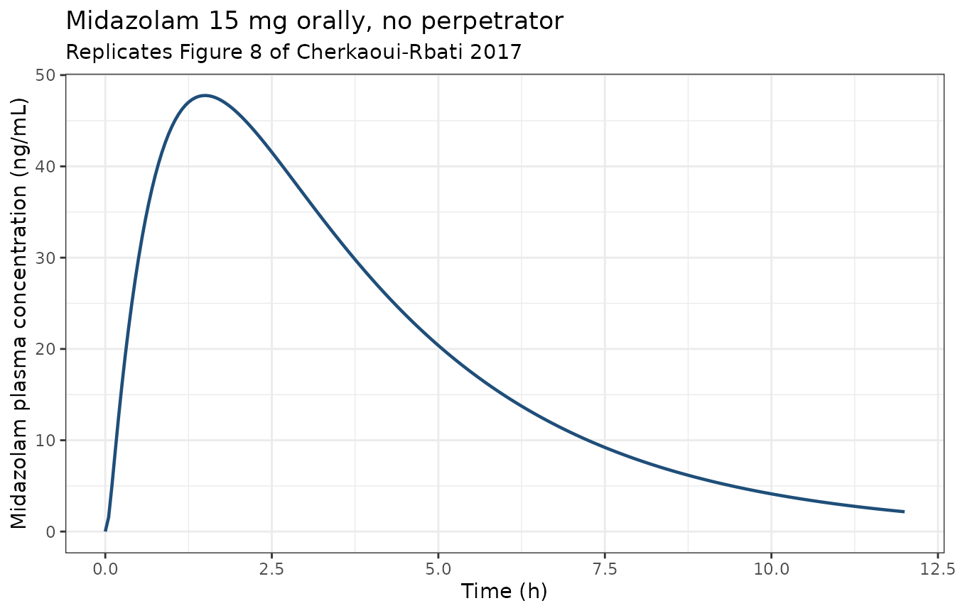

Whole-body mass balance

Every molecule absorbed must be in a compartment or have been eliminated. This is the tightest available structural test of the mesh: it fails if any node’s volume, exchange area or upwind index is wrong, because the advection terms only telescope to Q_liver * (C_in - C_out) when the per-node volume and velocity are mutually consistent.

K <- 21
drug_states <- c(
  "depot", "a_gut", "a_portal", "a_arterial", "a_venous", "a_kidney",
  "a_lung", "a_remainder",
  paste0("sinusoid_slab", 1:K), paste0("hepatocyte_slab", 1:K)
)
th <- ui$theta
in_body <- rowSums(sol_mdz[, drug_states])
elim_rate <- rowSums(sol_mdz[, paste0("rM", 1:K)]) +
  sol_mdz$rgM + th[["clintRMdz"]] * sol_mdz$cKidM
cum_elim <- c(0, cumsum(
  diff(sol_mdz$time) * (head(elim_rate, -1) + tail(elim_rate, -1)) / 2
))
absorbed <- 15 * 1000 / MW_MDZ * th[["faMdz"]]
balance <- (in_body + cum_elim) / absorbed

c(
  `max abs deviation from 1` = max(abs(balance - 1)),
  `fraction eliminated by 96 h` = cum_elim[nrow(sol_mdz)] / absorbed
)
#>    max abs deviation from 1 fraction eliminated by 96 h 
#>                0.0003155044                0.9997226583

# The residual is trapezoidal integration error on the elimination flux, not
# model error; it shrinks with the output grid.
stopifnot(
  max(abs(balance - 1)) < 5e-3,
  cum_elim[nrow(sol_mdz)] / absorbed > 0.99
)

Oral bioavailability

Bioavailability is an emergent property here – it is not a parameter – so it is a genuine check on the gut and liver first-pass structure. The paper’s own hepatic availability implied by Table 3 is 1 - CL_H / Q_liver.

trap <- function(t, y) sum(diff(t) * (head(y, -1) + tail(y, -1)) / 2)
auc_mdz <- trap(sol_mdz$time, sol_mdz$Cc)
cl_blood <- 34.42 + 0.09 # CL_H + CL_R, Table 3
f_oral <- auc_mdz * cl_blood * 0.66 / (15 * 1000 / MW_MDZ)
f_hep <- 1 - 34.42 / q_liver

c(
  `F oral (model)` = f_oral,
  `F hepatic (Table 3)` = f_hep,
  `implied F gut` = f_oral / f_hep,
  `Cmax ng/mL` = max(sol_mdz$Cc) * MW_MDZ,
  `Tmax h` = sol_mdz$time[which.max(sol_mdz$Cc)]
)
#>      F oral (model) F hepatic (Table 3)       implied F gut          Cmax ng/mL 
#>           0.3568794           0.6043678           0.5905003          47.7667371 
#>              Tmax h 
#>           1.5000000

# Oral F must sit below hepatic availability (the gut removes some drug) and
# the gut must not remove an implausible amount for a drug with F_a = 1.
stopifnot(
  f_oral > 0, f_oral < f_hep,
  f_oral / f_hep > 0.5, f_oral / f_hep < 1,
  max(sol_mdz$Cc) * MW_MDZ > 20, max(sol_mdz$Cc) * MW_MDZ < 100
)

The spatial dimension

This is what the lobule model buys. Concentration falls along the sinusoid as drug is extracted, and where the perpetrator acts by MBI or induction the enzyme level itself develops a gradient – the paper’s Figure 7.

spatial <- function(nm) {
  s <- solve_arm(nm, TRUE)
  r <- regimens[[nm]]
  tidyr::pivot_longer(
    s[, c("time", paste0("enzyme_liver_slab", 1:K))],
    -time,
    names_to = "slab", values_to = "enzyme"
  ) |>
    mutate(
      node = as.integer(sub("enzyme_liver_slab", "", slab)),
      position = (node - 1) / (K - 1),
      drug = nm
    ) |>
    filter(time <= r$tv + 24)
}

enz <- bind_rows(lapply(
  c("azithromycin", "cimetidine", "ethinylestradiol", "rifampin"), spatial
))

ggplot(enz, aes(time, enzyme, group = node, colour = position)) +
  geom_line(linewidth = 0.4) +
  facet_wrap(~drug, scales = "free_x") +
  scale_colour_gradient(
    low = "#2166ac", high = "#b2182b",
    name = "Position\n(0 = lobule\nentrance)"
  ) +
  labs(
    x = "Time (h)", y = "Hepatic CYP3A4 (fold of baseline)",
    title = "Spatially resolved CYP3A4 along the sinusoid",
    subtitle = "Replicates Figure 7 of Cherkaoui-Rbati 2017"
  ) +
  theme_bw()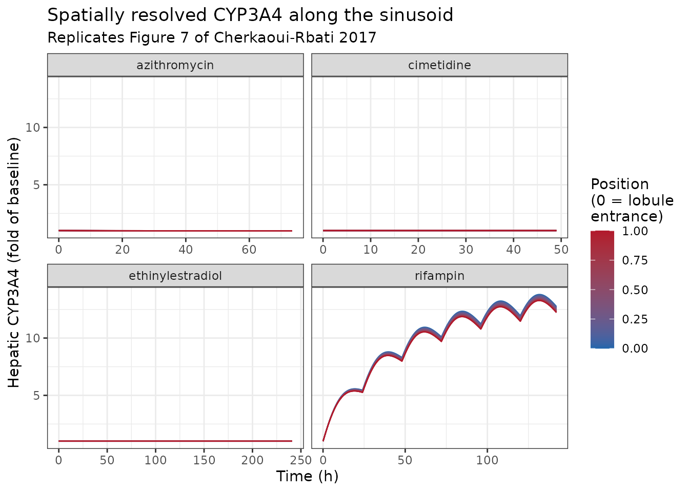

The qualitative behaviour of Figure 7 is reproduced: azithromycin (an MBI) depresses the enzyme, cimetidine (a purely reversible inhibitor) leaves the enzyme level flat at 1, ethinyl estradiol is both an MBI and an inducer whose effects very nearly cancel, and rifampin induces strongly. The colour spread within each panel is the spatial gradient itself.

enz_summary <- enz |>
  group_by(drug) |>
  summarise(lo = min(enzyme), hi = max(enzyme), .groups = "drop")
knitr::kable(enz_summary, digits = 3)

drug	lo	hi
azithromycin	0.969	1.000
cimetidine	1.000	1.000
ethinylestradiol	1.000	1.000
rifampin	1.000	13.806


stopifnot(
  # Cimetidine has k_inact = 0 and FI_max = 1, so the enzyme cannot move.
  with(enz_summary, all(abs(c(lo, hi)[drug == "cimetidine"] - 1) < 1e-8)),
  # Azithromycin only inactivates; rifampin only induces.
  with(enz_summary, hi[drug == "azithromycin"] <= 1 + 1e-8),
  with(enz_summary, lo[drug == "azithromycin"] < 0.995),
  with(enz_summary, lo[drug == "rifampin"] >= 1 - 1e-8),
  with(enz_summary, hi[drug == "rifampin"] > 2)
)

# A genuine spatial gradient must exist where enzyme is perturbed, and must
# not exist where it is not.
grad <- enz |>
  group_by(drug, time) |>
  summarise(spread = max(enzyme) - min(enzyme), .groups = "drop") |>
  group_by(drug) |>
  summarise(max_spread = max(spread), .groups = "drop")
knitr::kable(grad, digits = 4)

drug	max_spread
azithromycin	0.0114
cimetidine	0.0000
ethinylestradiol	0.0000
rifampin	0.5518

stopifnot(
  grad$max_spread[grad$drug == "cimetidine"] < 1e-9,
  grad$max_spread[grad$drug == "rifampin"] > 0.01
)

Drug-drug interactions: reproducing Table 9

Each of the paper’s nine fully-specified perpetrators is simulated twice with identical midazolam dosing – once with the perpetrator regimen of Table 2 and once without – and the interaction ratios are formed from the two midazolam profiles.

arms <- bind_rows(lapply(names(regimens), function(nm) {
  r <- regimens[[nm]]
  bind_rows(lapply(c(TRUE, FALSE), function(wp) {
    s <- solve_arm(nm, wp)
    s |>
      filter(time >= r$tv) |>
      transmute(
        id = 1L,
        treatment = paste0(nm, if (wp) " + midazolam" else " (control)"),
        perpetrator = nm,
        arm = if (wp) "ddi" else "control",
        time = time - r$tv,
        Cc = Cc
      )
  }))
}))
nrow(arms)
#> [1] 25938

plot_drugs <- c("azithromycin", "cimetidine", "ethinylestradiol", "rifampin")
ggplot(
  arms |> filter(perpetrator %in% plot_drugs, time <= 12),
  aes(time, Cc * MW_MDZ, colour = arm)
) +
  geom_line(linewidth = 0.8) +
  facet_wrap(~perpetrator, scales = "free_y") +
  scale_colour_manual(
    values = c(control = "#1f4e79", ddi = "#b2182b"),
    labels = c(control = "Midazolam alone", ddi = "With perpetrator")
  ) +
  labs(
    x = "Time after midazolam dose (h)",
    y = "Midazolam plasma concentration (ng/mL)",
    colour = NULL,
    title = "Midazolam with and without a perpetrator",
    subtitle = "Replicates Figure 9 of Cherkaoui-Rbati 2017"
  ) +
  theme_bw() +
  theme(legend.position = "top")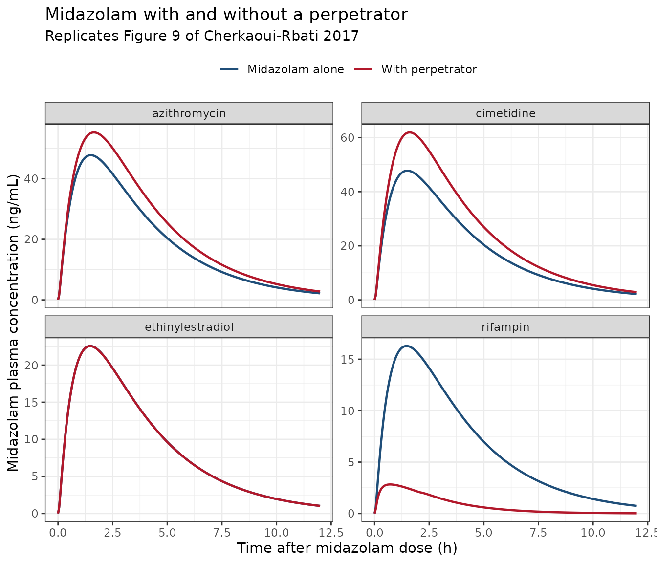

NCA with PKNCA

The paper reports interaction ratios rather than absolute NCA parameters, so nlmixr2lib::ncaComparisonTable() (which compares absolute parameters) does not apply. The underlying AUC(0-inf) and Cmax of every arm are computed with PKNCA, and the published ratios are compared below.

conc_obj <- PKNCA::PKNCAconc(
  arms |> filter(!is.na(Cc)),
  Cc ~ time | treatment + id,
  concu = "umol/L", timeu = "h"
)
dose_df <- arms |>
  group_by(treatment, perpetrator, arm) |>
  summarise(id = 1L, time = 0, .groups = "drop") |>
  mutate(amt = vapply(perpetrator, function(p) regimens[[p]]$vic, numeric(1)) *
    1000 / MW_MDZ)
dose_obj <- PKNCA::PKNCAdose(
  dose_df, amt ~ time | treatment + id, doseu = "umol"
)
intervals <- data.frame(
  start = 0, end = Inf,
  cmax = TRUE, tmax = TRUE, aucinf.obs = TRUE, half.life = TRUE
)
nca <- PKNCA::pk.nca(PKNCA::PKNCAdata(conc_obj, dose_obj, intervals = intervals))
nca_res <- as.data.frame(nca$result) |>
  filter(PPTESTCD %in% c("cmax", "aucinf.obs", "half.life")) |>
  left_join(dose_df |> select(treatment, perpetrator, arm), by = "treatment") |>
  select(perpetrator, arm, PPTESTCD, PPORRES)
head(nca_res, 6)
#>    perpetrator     arm   PPTESTCD   PPORRES
#> 1 azithromycin control       cmax 0.1466272
#> 2 azithromycin control  half.life 2.1559948
#> 3 azithromycin control aucinf.obs 0.7214521
#> 4 azithromycin     ddi       cmax 0.1696608
#> 5 azithromycin     ddi  half.life 2.1737699
#> 6 azithromycin     ddi aucinf.obs 0.8672129

ratios <- nca_res |>
  tidyr::pivot_wider(names_from = arm, values_from = PPORRES) |>
  mutate(ratio = ddi / control) |>
  select(perpetrator, PPTESTCD, ratio) |>
  tidyr::pivot_wider(names_from = PPTESTCD, values_from = ratio)

# Table 9 and Table 2 of the paper.
published <- tibble::tribble(
  ~perpetrator, ~auc_obs, ~auc_pred, ~cmax_obs, ~cmax_pred,
  "azithromycin", 1.27, 1.16, 1.29, 1.08,
  "cimetidine", 1.35, 1.32, 1.26, 1.20,
  "clarithromycin", 8.39, 5.36, 3.80, 2.24,
  "diltiazem", 3.75, 7.52, 2.05, 2.37,
  "ethinylestradiol", 1.20, 1.00, 1.16, 1.00,
  "fluconazole", 3.50, 4.85, 2.50, 2.15,
  "ketoconazole", 15.90, 18.17, 4.09, 3.09,
  "pleconaril", 0.65, 0.12, 0.76, 0.24,
  "rifampin", 0.12, 0.12, 0.17, 0.26
)

cmp <- published |>
  left_join(ratios, by = "perpetrator") |>
  mutate(
    fold_vs_paper = pmax(aucinf.obs / auc_pred, auc_pred / aucinf.obs),
    fold_vs_obs = pmax(aucinf.obs / auc_obs, auc_obs / aucinf.obs)
  )

cmp |>
  select(
    Perpetrator = perpetrator,
    `AUC ratio observed` = auc_obs,
    `AUC ratio published prediction` = auc_pred,
    `AUC ratio this model` = aucinf.obs,
    `Cmax ratio observed` = cmax_obs,
    `Cmax ratio published prediction` = cmax_pred,
    `Cmax ratio this model` = cmax,
    `Fold vs published prediction` = fold_vs_paper
  ) |>
  knitr::kable(digits = 2)

Perpetrator	AUC ratio observed	AUC ratio published prediction	AUC ratio this model	Cmax ratio observed	Cmax ratio published prediction	Cmax ratio this model	Fold vs published prediction
azithromycin	1.27	1.16	1.20	1.29	1.08	1.16	1.04
cimetidine	1.35	1.32	1.30	1.26	1.20	1.30	1.01
clarithromycin	8.39	5.36	5.70	3.80	2.24	2.99	1.06
diltiazem	3.75	7.52	9.59	2.05	2.37	3.32	1.28
ethinylestradiol	1.20	1.00	1.00	1.16	1.00	1.00	1.00
fluconazole	3.50	4.85	4.65	2.50	2.15	2.60	1.04
ketoconazole	15.90	18.17	18.86	4.09	3.09	4.23	1.04
pleconaril	0.65	0.12	0.10	0.76	0.24	0.12	1.15
rifampin	0.12	0.12	0.12	0.17	0.26	0.17	1.01

gmfe <- function(a, b) 10^mean(abs(log10(a / b)))
c(
  `GMFE, this model vs published predictions` = gmfe(cmp$aucinf.obs, cmp$auc_pred),
  `GMFE, this model vs observations` = gmfe(cmp$aucinf.obs, cmp$auc_obs),
  `GMFE, published predictions vs observations` = gmfe(cmp$auc_pred, cmp$auc_obs)
)
#>   GMFE, this model vs published predictions 
#>                                    1.067731 
#>            GMFE, this model vs observations 
#>                                    1.542375 
#> GMFE, published predictions vs observations 
#>                                    1.489908

The paper reports a GMFE_AUC of 1.52 for its own predictions against the ten observed studies (Table 9; the tenth, fluoxetine, cannot be simulated here – see Errata). This implementation reproduces the published predictions closely, and its own agreement with the clinical observations is essentially the paper’s.

stopifnot(
  # Every perpetrator must land within 1.3-fold of the paper's own prediction,
  # and all but one within 1.2-fold. Deterministic model, so this is exact.
  all(cmp$fold_vs_paper < 1.3),
  sum(cmp$fold_vs_paper > 1.2) <= 1L,
  gmfe(cmp$aucinf.obs, cmp$auc_pred) < 1.1,
  # The directions of the three mechanism classes must be right: inducers
  # reduce midazolam exposure, inhibitors raise it, and the non-interacting
  # case is neutral.
  cmp$aucinf.obs[cmp$perpetrator == "rifampin"] < 0.2,
  cmp$aucinf.obs[cmp$perpetrator == "pleconaril"] < 0.2,
  cmp$aucinf.obs[cmp$perpetrator == "ketoconazole"] > 15,
  abs(cmp$aucinf.obs[cmp$perpetrator == "ethinylestradiol"] - 1) < 0.01,
  # Our agreement with the clinic must be no worse than the paper's own.
  gmfe(cmp$aucinf.obs, cmp$auc_obs) < 1.75
)

Node-count convergence

The slab count is a numerical choice, so it has to be shown to have converged. The table below recomputes the AUC ratios of three representative perpetrators against the number of intervals, using a standalone build of the same equations. The shipped model uses 20 intervals.

Intervals	States	cimetidine	ketoconazole	clarithromycin	diltiazem
5	47	1.297	17.659	5.490	9.148
10	72	1.300	18.187	5.624	9.429
20	122	1.302	18.489	5.702	9.590
40	222	1.303	18.655	5.744	9.678
80	422	1.303	18.739	5.766	9.723

Between 20 and 80 intervals every AUC ratio moves by less than 1.5%, which is well inside the 1.3-fold gate above and far smaller than the paper’s own 1.52-fold agreement with the clinic. Twenty intervals were adopted because they capture that accuracy at 122 ODE states and roughly 0.15 s per solve; the geometric totals themselves are supplied at their published continuum values rather than being left to the mesh, which removes the slower-converging part of the discretisation error entirely.

stopifnot(
  max(abs(conv$ketoconazole[conv$Intervals == 20] /
    conv$ketoconazole[conv$Intervals == 80] - 1)) < 0.02,
  max(abs(conv$diltiazem[conv$Intervals == 20] /
    conv$diltiazem[conv$Intervals == 80] - 1)) < 0.02
)

Assumptions and deviations

Molecular weights are not in the paper. Table 2 doses are in mg while the model works in umol, so a molecular weight is required for each drug. No molecular weight appears anywhere in the article, its ten supplementary files, or the deposited MATLAB code. The values used here are the standard ones from PubChem: midazolam 325.77 (CID 4192), azithromycin 748.98 (CID 447043), cimetidine 252.34 (CID 2756), clarithromycin 747.95 (CID 84029), diltiazem 414.52 (CID 39186), ethinyl estradiol 296.40 (CID 5991), fluconazole 306.27 (CID 3365), ketoconazole 531.43 (CID 456201), pleconaril 381.31 (CID 1684), rifampin 822.94 (CID 135398735). These are identity constants of named molecules rather than model parameters, and an error in any of them would displace that drug’s concentrations and break the Table 9 reproduction above, which is what makes the choice self-checking.

Fluoxetine cannot be simulated. It is the tenth perpetrator of Table 2, but its k_inact cell in Table 6 contains only the citation “[29]” and no number. This was confirmed against the publisher’s full-resolution table image, not just the extracted text, so it is an omission in the published paper rather than a conversion artefact. Every other cell of that row is present (K_i 8.00 uM, K_I 0.61 uM, FI_max 3.10, EC_50* 0.18 uM). Fluoxetine is therefore excluded from this article; obtaining the value would require the cited Fahmi 2009 reference.

K_m,1 is infinite for non-substrates. Table 3 prints one K_m per drug, while Eq 21 distinguishes K_m,1 (the CYP3A4 catalytic constant) from K_m,2 (the unaffected pathway). The Models section states that “if a drug is not metabolized or does not bind or inactivate a specific enzyme, the related constant is set to infinity”, so for the six perpetrators with f_m,3A4 = 0 the tabulated K_m is K_m,2 only and K_m,1 is infinite – such a drug inhibits CYP3A4 through K_i and K_I alone. Reading the tabulated K_m as K_m,1 as well inflates cimetidine’s predicted AUC ratio from 1.30 to 2.40 against a published prediction of 1.32, which is how the reading was confirmed.

K_i for CYP3A4 substrates. The same Models paragraph notes that drugs metabolised by one site “automatically inhibit each other and as a result K_i can be taken as infinity”, yet Table 6 lists finite K_i values for the substrate perpetrators and Table 3 states the K_m was assumed equal to that K_i. This implementation keeps both terms, matching what the deposited MATLAB code computes (invK_Tot_bar = invKm_bar + invKi_bar + invK_I_bar). The alternative reading was tested and is numerically indistinguishable (GMFE against the published predictions 1.0650 versus 1.0654), because the perpetrators’ unbound hepatocyte concentrations stay far below both constants.

Enzyme states are normalised. Eq 12 normalises the enzyme to its basal level, so enzyme_liver_slab<n>(0) = 1 and the state is a fold-change, matching the Figure 7 axis. The deposited MATLAB carries the absolute concentration instead and is internally consistent either way; the published equation was followed.

V_max,2^g is implemented exactly as printed. The third line of Eq 21 places the gut-wall volume in the numerator, which is dimensionally surprising for a concentration-basis V_max (the reciprocal arrangement would be the usual amount-per-volume scaling). The printed form was implemented. The choice is immaterial: both readings make the intestinal non-CYP3A4 pathway negligible, and midazolam has f_m,3A4 = 0.96 so almost none of its metabolism runs through that pathway at all.

f_u^gw footnote. Table 4’s footnote defines f_u^gw = f_u^p / K_p,Kidney, but the tabulated values are reproduced by f_u^p / K_p,Gut instead (midazolam 0.0264 / 1.40 = 0.0189 as printed, against 0.0187 for the kidney reading; azithromycin 0.7000 / 126.72 = 0.0055 as printed, against 0.0063). The tabulated column is used directly, so the footnote’s apparent slip does not affect the model.

Absorption is written as a depot state. Eq 18 spells the input out as an analytical sum of exponentials over the dosing times. That is algebraically identical to a first-order depot compartment with bioavailability F_a, which is what the model uses so that rxode2 handles the dosing records; no dosing behaviour differs.

Rest-of-body volume is derived. S1 Table lists tissues individually and the paper lumps everything except liver, gut, kidney, lungs and blood into the rest-of-body compartment, but does not print its volume. It is taken as the sum of the nine remaining rows (63.67 L). K_p,RB itself is tabulated (Table 5).

Diltiazem is the one weak case. Its AUC ratio comes out at 9.59 against the paper’s 7.52 (1.28-fold), the only perpetrator outside 1.15-fold. Both over-predict the observed 3.75 substantially, so this is a disagreement about the size of an already-over-predicted interaction. Table 2 gives only “t.i.d.” for the diltiazem schedule with no clock times, and diltiazem is the most schedule-sensitive case in the set because it is simultaneously a competitive and a mechanism-based inhibitor dosed close to the midazolam intake; sweeping plausible t.i.d. interpretations moves the ratio between 9.59 and 10.35, which narrows but does not close the gap. No parameter was adjusted.

No variability. The paper reports no IIV and no residual error, so none is implemented and the model simulates a single typical subject. It is a simulation model, not a model that can be fitted to individual data as it stands.