Capecitabine + docetaxel tumor growth inhibition, PFS and survival in metastatic breast cancer (Bruno 2012)
Source:vignettes/articles/Bruno_2012_capecitabine_docetaxel_mbc.Rmd
Bruno_2012_capecitabine_docetaxel_mbc.RmdModel and source
Bruno 2012 built a three-part modeling framework to work out which capecitabine starting dose, combined with docetaxel, would be noninferior to the registered 1,250 mg/m^2 dose in second-line metastatic breast cancer. The framework has three independently fitted models, extracted here as three model files:
-
Bruno_2012_capecitabine_docetaxel_tgi– longitudinal tumor growth inhibition (TGI) model, NONMEM VI, Supplementary Information + Supplementary Table S1. -
Bruno_2012_capecitabine_docetaxel_os– log-normal parametric overall survival model, S-PLUScensorReg, Table 1. -
Bruno_2012_capecitabine_docetaxel_pfs– log-normal parametric progression-free survival model, S-PLUScensorReg, Table 2.
The two survival models are drug-independent: their only treatment-dependent input is the model-predicted relative change from baseline in tumor size at week 6 (end of cycle 2), so any TGI model can drive them.
- Article: https://doi.org/10.1038/psp.2012.20 (open access, PMC3600724)
- Supplement: Supplementary Information (model equations, inter-patient variability and residual-error forms, and the full NONMEM control stream) and Supplementary Table S1 (TGI final parameter estimates), both accompanying the article on the journal website and mirrored in PMC.
tgi_fun <- readModelDb("Bruno_2012_capecitabine_docetaxel_tgi")
os_fun  <- readModelDb("Bruno_2012_capecitabine_docetaxel_os")
pfs_fun <- readModelDb("Bruno_2012_capecitabine_docetaxel_pfs")

cat(tgi_fun()$reference)
#> Bruno R, Lindbom L, Schaedeli Stark F, Chanu P, Gilberg F, Frey N, Claret L. Simulations to assess phase II noninferiority trials of different doses of capecitabine in combination with docetaxel for metastatic breast cancer. CPT Pharmacometrics Syst Pharmacol. 2012;1(12):e19. doi:10.1038/psp.2012.20. Structural equations, parameter definitions and the NONMEM control stream are in the Supplementary Information; final parameter estimates are in Supplementary Table S1.
Population
The TGI model was fitted to a pooled longitudinal tumor-size database of 888 patients with locally advanced or metastatic breast cancer: 463 from the pivotal phase III study SO14999 and 425 from the randomized phase II noninferiority study NO16853. Those patients contributed 2,988 tumor-size observations, a mean of 3.4 measurements per patient, and baseline tumor size (sum of the longest diameters) ranged from 10 to 520 mm.
The same 888 patients supported both survival models. 556 (63%) died during the observation period, with a median (95% CI) survival of 14.8 months (13.6-16.0); 790 (89%) progressed or died, with a median PFS of 5.8 months (5.5-6.3). ECOG performance status was 1 rather than 0 in 319 patients (36%), and 687 (77%) had more than one metastatic site. Estrogen- and progesterone-receptor status were missing in 220 patients (25%), which is why those covariates were dropped from the final models. Bruno 2012 does not tabulate age, weight, sex or race for this cohort.
Tumor response used WHO criteria in SO14999 and RECIST in NO16853; that difference is one of the reasons the authors give for the study effect that both survival models retain.
str(tgi_fun()$population)
#> List of 7
#>  $ species       : chr "human"
#>  $ n_subjects    : int 888
#>  $ n_studies     : int 2
#>  $ n_observations: int 2988
#>  $ disease_state : chr "locally advanced / metastatic breast cancer, second line after anthracycline pretreatment"
#>  $ dose_range    : chr "capecitabine 825 or 1,250 mg/m^2 twice daily on days 1-14 of each 3-week cycle plus docetaxel 75 mg/m^2 on day "| __truncated__
#>  $ notes         : chr "Pooled longitudinal tumor-size database of 888 patients (463 from the pivotal phase III study SO14999, 425 from"| __truncated__
Source trace
Every ini() entry in the three model files carries an
in-file comment naming its source location. They are collected here for
review.
Tumor growth inhibition model
| Equation / parameter | Value | Source location |
|---|---|---|
lkgrow (KL) |
0.00437 /week | Suppl. Table S1, RSE 15%; $THETA(1)
|
lkkill_docetaxel (KD,0,Doc) |
0.00128 | Suppl. Table S1, RSE 31%; $THETA(2)
|
lkkill_capecitabine (KD,0,Cap) |
0.00470 | Suppl. Table S1, RSE 20%; $THETA(3)
|
lres_docetaxel (lambda_Doc) |
0.0450 /week | Suppl. Table S1, RSE 39%; $THETA(4)
|
lres_capecitabine (lambda_Cap) |
0.240 /week | Suppl. Table S1, RSE 23%; $THETA(5)
|
lkel_docetaxel (KP,Doc) |
0.1 /week, FIXED | Suppl. Table S1 “Fixed”; $THETA(7) 0.1 FIXED
|
lkel_capecitabine (KP,Cap) |
3 /week, FIXED | Suppl. Table S1 “Fixed”; $THETA(8) 3 FIXED
|
etalkgrow |
omega^2 = 1.60 | Suppl. Table S1, RSE 5% |
etalkkill_docetaxel |
omega^2 = 1.31 | Suppl. Table S1, RSE 15% |
etalkkill_capecitabine |
omega^2 = 1.30 | Suppl. Table S1, RSE 19% |
addSdStudySO14999 |
sqrt(332) = 18.22 mm | Suppl. Table S1 sigma^2 = 332 mm^2, RSE 11%;
$THETA(6)
|
addSdStudyNO16853 |
sqrt(112) = 10.58 mm | Suppl. Table S1 sigma^2 = 112 mm^2, RSE 18%;
$THETA(9)
|
| ODE system, K-PD biophase + additive drug effects | n/a | Suppl. Information equations and $DES block |
tumor_size(0) <- TUM_SLD |
n/a |
$PK: A_0(3) = BASE
|
| study-selected additive residual error | n/a |
$ERROR: Y = F + REE*ERR(1),
IF(STUD.EQ.2) REE = SQRT(THETA(9))
|
Overall survival model
| Parameter | Value | Source location |
|---|---|---|
ltmed0 (beta_0) |
3.02 | Table 1, RSE 5%, 95% CI 2.72-3.31 |
e_tumsld_tmed (beta_1) |
-0.00231 /mm | Table 1, RSE 19%, 95% CI -0.00316 to -0.00146 |
e_rcfb6sld_tmed (beta_2) |
-0.801 | Table 1, RSE 17%, 95% CI -1.060 to -0.541 |
e_whops_tmed (beta_3) |
-0.352 | Table 1, RSE 17%, 95% CI -0.468 to -0.236 |
e_metge2_tmed (beta_4) |
-0.200 | Table 1, RSE 36%; footnote c gives the 1/2 coding |
e_studyno16853_tmed (beta_5) |
0.131 | Table 1, RSE 44%; footnote c gives the 1/2 coding |
sdlogt (sigma) |
0.773 | Table 1, “Random variability” |
| log-normal AFT form | n/a | Suppl. Information survival-model equation |
Progression-free survival model
| Parameter | Value | Source location |
|---|---|---|
ltmed0 (beta_0) |
1.38 | Table 2, RSE 7%, 95% CI 1.20-1.56 |
e_tumsld_tmed (beta_1) |
-0.00165 /mm | Table 2, RSE 26%, 95% CI -0.00248 to -0.00082 |
e_rcfb6sld_tmed (beta_2) |
-1.18 | Table 2, RSE 11%, 95% CI -1.43 to -0.92 |
e_whops_tmed (beta_3) |
-0.195 | Table 2, RSE 29%; printed CI has a typesetting error, see Errata |
e_studyno16853_tmed (beta_4) |
0.216 | Table 2, RSE 26%, 95% CI 0.107-0.325; footnote c gives the 1/2 coding |
sdlogt (sigma) |
0.799 | Table 2, “Random variability” |
Check 1: the survival models reproduce the paper’s own worked examples
Bruno 2012 Results quote four expected event times as a function of the week-6 fractional change in tumor size:
- overall survival: 11.8 months (95% CI 10.1-14.0) at a 30% tumor-size progression, 19.3 months (17.3-21.6) at a 30% shrinkage (Supplementary Figure S5);
- PFS: 3.8 months (3.2-4.5) at a 30% progression, 7.7 months (7.1-8.5) at a 30% shrinkage (Supplementary Figure S8).
The ratio of the two values within each model depends only on beta_2, so it is a covariate-free transcription check on the single most influential coefficient in each model.
os_par  <- rxode2::rxode2(os_fun)$theta
pfs_par <- rxode2::rxode2(pfs_fun)$theta

ratio_chk <- tibble::tibble(
  model     = c("Overall survival", "Progression-free survival"),
  published = c(19.3 / 11.8, 7.7 / 3.8),
  model_ratio = c(exp(-os_par[["e_rcfb6sld_tmed"]] * 0.6),
                  exp(-pfs_par[["e_rcfb6sld_tmed"]] * 0.6))
) |>
  mutate(pct_diff = 100 * (model_ratio - published) / published)

ratio_chk |>
  rename("Model" = model,
         "Published ratio (shrinkage / progression)" = published,
         "Model ratio" = model_ratio,
         "Difference (%)" = pct_diff) |>
  knitr::kable(digits = 4,
caption = "Ratio of the published expected event times at -30% versus +30% week-6 tumor-size change. Depends only on beta_2.")| Model | Published ratio (shrinkage / progression) | Model ratio | Difference (%) |
|---|---|---|---|
| Overall survival | 1.6356 | 1.6170 | -1.1341 |
| Progression-free survival | 2.0263 | 2.0299 | 0.1782 |
# Deterministic: no random numbers are involved, so a tight bound is correct.
stopifnot(all(abs(ratio_chk$pct_diff) < 3))
The absolute values additionally pin down the reference patient the figures were drawn at. Bruno 2012 states that the clinical trial simulations were conditioned on study NO16853, and 77% of the cohort had more than one metastatic site; solving the PFS relation for the remaining unknown gives a baseline tumor size of about 75 mm, which then reproduces all four published values.
reference_patient <- tibble::tibble(
  TUM_SLD       = 75,   # inferred by inversion, see Errata
  WHO_PS        = 0,
  MET_GE2       = 1,
  STUDY_NO16853 = 1
)

eval_surv <- function(model_fun, rcfb6) {
  mod <- rxode2::rxode2(model_fun)
  ev <- reference_patient[rep(1, length(rcfb6)), ]
  ev$id        <- seq_along(rcfb6)
  ev$time      <- 0
  ev$evid      <- 0
  ev$RCFB6_SLD <- rcfb6
  as.data.frame(rxode2::rxSolve(mod, events = as.data.frame(ev)))$tmed
}

worked <- tibble::tibble(
  endpoint  = c("Overall survival", "Overall survival",
                "Progression-free survival", "Progression-free survival"),
  rcfb6     = c(0.30, -0.30, 0.30, -0.30),
  published = c(11.8, 19.3, 3.8, 7.7),
  model     = c(eval_surv(os_fun,  c(0.30, -0.30)),
                eval_surv(pfs_fun, c(0.30, -0.30)))
) |>
  mutate(pct_diff = 100 * (model - published) / published)

worked |>
  rename("Endpoint" = endpoint,
         "Week-6 tumor-size change" = rcfb6,
         "Published median (months)" = published,
         "Model median (months)" = model,
         "Difference (%)" = pct_diff) |>
  knitr::kable(digits = 3,
caption = "Bruno 2012 Results worked examples versus the packaged models at the inferred reference patient.")| Endpoint | Week-6 tumor-size change | Published median (months) | Model median (months) | Difference (%) |
|---|---|---|---|---|
| Overall survival | 0.3 | 11.8 | 11.804 | 0.035 |
| Overall survival | -0.3 | 19.3 | 19.088 | -1.099 |
| Progression-free survival | 0.3 | 3.8 | 3.797 | -0.075 |
| Progression-free survival | -0.3 | 7.7 | 7.708 | 0.103 |
Check 2: the log-normal survival function is internally consistent
For a log-normal accelerated-failure-time model, exp(mu)
is by construction the median survival time, so surv(tmed)
must equal exactly 0.5, and the model must be a proper survival function
(monotone, surv(0) = 1).
check_lognormal <- function(model_fun) {
  mod <- rxode2::rxode2(model_fun)
  ev <- reference_patient
  ev$id <- 1L; ev$evid <- 0L; ev$RCFB6_SLD <- -0.10
  tmed <- as.data.frame(rxode2::rxSolve(
    mod, events = as.data.frame(dplyr::mutate(ev, time = 0))))$tmed[1]
  grid <- as.data.frame(rxode2::rxSolve(
    mod,
    events = as.data.frame(dplyr::mutate(ev[rep(1, 61), ],
                                         time = c(0, tmed, seq(0.5, 60, length.out = 59))))))
  grid <- grid[order(grid$time), ]
  list(
    at_median = grid$surv[which.min(abs(grid$time - tmed))],
    at_zero   = grid$surv[1],
    monotone  = all(diff(grid$surv) <= 1e-12)
  )
}

lognorm_chk <- lapply(list(OS = os_fun, PFS = pfs_fun), check_lognormal)
str(lognorm_chk)
#> List of 2
#>  $ OS :List of 3
#>   ..$ at_median: num 0.5
#>   ..$ at_zero  : num 1
#>   ..$ monotone : logi TRUE
#>  $ PFS:List of 3
#>   ..$ at_median: num 0.5
#>   ..$ at_zero  : num 1
#>   ..$ monotone : logi TRUE

stopifnot(
  abs(lognorm_chk$OS$at_median  - 0.5) < 1e-6,
  abs(lognorm_chk$PFS$at_median - 0.5) < 1e-6,
  abs(lognorm_chk$OS$at_zero  - 1) < 1e-9,
  abs(lognorm_chk$PFS$at_zero - 1) < 1e-9,
  lognorm_chk$OS$monotone,
  lognorm_chk$PFS$monotone
)
Virtual cohort and dosing
The original patient-level data are not public. The cohort below approximates the published trial demographics: baseline tumor size log-normally distributed with a median of 75 mm truncated to the reported 10-520 mm range, ECOG 1 in 36% of subjects, more than one metastatic site in 77%, and every subject assigned to study NO16853 (the study Bruno 2012 conditioned its simulations on).
Four arms are simulated, matching the dose levels Bruno 2012 studied: docetaxel alone, and docetaxel plus capecitabine at 825, 1,000 and 1,250 mg/m^2 twice daily. Capecitabine is given on days 1-14 of each 3-week cycle and docetaxel on day 1; two cycles (6 weeks) are needed to reach the week-6 tumor assessment. Body surface area is not reported in Bruno 2012 and is held at 1.7 m^2 (see Errata).
# set.seed() seeds R's RNG; rxSetSeed() seeds rxode2's, which is partitioned per
# solver thread. Neither makes the draw identical across machines with different
# thread counts, so every assertion below is written to hold for any cohort the
# model can produce.
set.seed(20120026)
rxode2::rxSetSeed(20120026)

n_per_arm <- 200L
bsa       <- 1.7     # m^2; not reported by Bruno 2012, see Errata
cycle_wk  <- 3       # weeks per treatment cycle
n_cycles  <- 2
horizon   <- 6       # weeks; the week-6 (end of cycle 2) assessment

arms <- tibble::tribble(
  ~arm,                       ~cape_mgm2,
  "Docetaxel alone",          0,
  "Cape 825 + docetaxel",     825,
  "Cape 1000 + docetaxel",    1000,
  "Cape 1250 + docetaxel",    1250
)

# Capecitabine: twice daily on days 1-14 of each cycle; docetaxel: day 1.
cape_times <- as.vector(outer(seq(0, 13.5, by = 0.5) / 7,
                              (seq_len(n_cycles) - 1) * cycle_wk, "+"))
doc_times  <- (seq_len(n_cycles) - 1) * cycle_wk
obs_times  <- sort(unique(c(seq(0, horizon, by = 0.25), horizon)))

make_subjects <- function(n, id_offset = 0L) {
  sld <- pmin(pmax(rlnorm(n, meanlog = log(75), sdlog = 0.55), 10), 520)
  tibble::tibble(
    id            = id_offset + seq_len(n),
    TUM_SLD       = sld,
    WHO_PS        = rbinom(n, 1, 0.36),
    MET_GE2       = rbinom(n, 1, 0.77),
    STUDY_NO16853 = 1
  )
}

make_arm_events <- function(subjects, cape_mgm2, arm_label) {
  doses <- dplyr::bind_rows(
    tidyr::expand_grid(subjects, time = doc_times) |>
      dplyr::mutate(evid = 1L, amt = 75 * bsa, cmt = "depot_kpd_docetaxel"),
    if (cape_mgm2 > 0) {
      tidyr::expand_grid(subjects, time = cape_times) |>
        dplyr::mutate(evid = 1L, amt = cape_mgm2 * bsa,
                      cmt = "depot_kpd_capecitabine")
    } else NULL
  )
  obs <- tidyr::expand_grid(subjects, time = obs_times) |>
    dplyr::mutate(evid = 0L, amt = NA_real_, cmt = "tumor_size")
  dplyr::bind_rows(doses, obs) |>
    dplyr::mutate(arm = arm_label) |>
    dplyr::arrange(id, time, dplyr::desc(evid)) |>
    as.data.frame()
}

subjects <- make_subjects(n_per_arm)
events <- dplyr::bind_rows(lapply(seq_len(nrow(arms)), function(i) {
  s <- subjects
  s$id <- s$id + (i - 1L) * n_per_arm
  make_arm_events(s, arms$cape_mgm2[i], arms$arm[i])
}))

stopifnot(!anyDuplicated(unique(events[, c("id", "time", "evid")])))
Check 3: the ODE solution matches a hand-derived closed form
With every subject at the typical value the model is a linear
first-order biophase feeding an exponential-growth tumor state, so the
tumor-size trajectory has an exact closed form. Integrating the kill
term for a series of doses of amount D_j given at times
t_j,
log(y(T) / y(0)) = KL * T - sum_X KD_X * KP_X * sum_j D_j * exp(-lambda_X * t_j)
                            * (1 - exp(-(KP_X + lambda_X) * (T - t_j))) / (KP_X + lambda_X)
with the capecitabine doses divided by 1,000 to match the g^-1 unit of KD,0,Cap. Both sides use the same parameter values, so the only difference is ODE solver error and a tight bound is the correct assertion.
tgi_mod <- rxode2::rxode2(tgi_fun)
#> ℹ parameter labels from comments will be replaced by 'label()'
th <- tgi_mod$theta
p <- list(
  kgrow    = exp(th[["lkgrow"]]),
  kd_doc   = exp(th[["lkkill_docetaxel"]]),
  kd_cap   = exp(th[["lkkill_capecitabine"]]),
  res_doc  = exp(th[["lres_docetaxel"]]),
  res_cap  = exp(th[["lres_capecitabine"]]),
  kel_doc  = exp(th[["lkel_docetaxel"]]),
  kel_cap  = exp(th[["lkel_capecitabine"]])
)

kill_integral <- function(tt, dose, dose_times, kel, res) {
  vapply(tt, function(T) {
    j <- dose_times <= T
    if (!any(j)) return(0)
    sum(dose * exp(-res * dose_times[j]) *
          (1 - exp(-(kel + res) * (T - dose_times[j]))) / (kel + res))
  }, numeric(1))
}

closed_form <- function(tt, sld0, cape_mgm2) {
  i_doc <- p$kd_doc * p$kel_doc *
    kill_integral(tt, 75 * bsa, doc_times, p$kel_doc, p$res_doc)
  i_cap <- if (cape_mgm2 > 0) {
    p$kd_cap * (p$kel_cap / 1000) *
      kill_integral(tt, cape_mgm2 * bsa, cape_times, p$kel_cap, p$res_cap)
  } else 0
  sld0 * exp(p$kgrow * tt - i_doc - i_cap)
}

typ_subject <- tibble::tibble(id = 1L, TUM_SLD = 75, WHO_PS = 0,
                              MET_GE2 = 1, STUDY_NO16853 = 1)
typ_events <- dplyr::bind_rows(lapply(seq_len(nrow(arms)), function(i) {
  s <- typ_subject
  s$id <- i
  make_arm_events(s, arms$cape_mgm2[i], arms$arm[i])
}))

sim_typ <- rxode2::rxSolve(rxode2::zeroRe(tgi_mod), events = typ_events,
                           omega = NA, sigma = NA, keep = "arm") |>
  as.data.frame() |>
  dplyr::left_join(dplyr::select(arms, arm, cape_mgm2), by = "arm") |>
  dplyr::group_by(arm) |>
  dplyr::mutate(analytic = closed_form(time, 75, dplyr::first(cape_mgm2))) |>
  dplyr::ungroup() |>
  dplyr::mutate(rel_err = abs(tumor_size - analytic) / analytic)
#> Warning: No sigma parameters in the model

sim_typ |>
  dplyr::group_by(arm) |>
  dplyr::summarise("Max relative error" = max(rel_err), .groups = "drop") |>
  dplyr::rename("Arm" = arm) |>
  knitr::kable(digits = 12,
caption = "ODE solution versus the closed-form solution, typical values.")| Arm | Max relative error |
|---|---|
| Cape 1000 + docetaxel | 7.834470e-07 |
| Cape 1250 + docetaxel | 1.028571e-06 |
| Cape 825 + docetaxel | 6.246060e-07 |
| Docetaxel alone | 3.797840e-07 |
Check 4: dose-response ordering at typical values
Increasing the capecitabine starting dose must monotonically increase the predicted week-6 tumor shrinkage. At typical values this is deterministic.
wk6_typ <- sim_typ |>
  dplyr::filter(abs(time - horizon) < 1e-9) |>
  dplyr::transmute(arm, cape_mgm2, rcfb6 = tumor_size / 75 - 1) |>
  dplyr::arrange(cape_mgm2)

wk6_typ |>
  dplyr::rename("Arm" = arm,
                "Capecitabine (mg/m^2 BID)" = cape_mgm2,
                "Week-6 relative change from baseline" = rcfb6) |>
  knitr::kable(digits = 4,
caption = "Typical-value week-6 tumor-size change by arm.")| Arm | Capecitabine (mg/m^2 BID) | Week-6 relative change from baseline |
|---|---|---|
| Docetaxel alone | 0 | -0.0712 |
| Cape 825 + docetaxel | 825 | -0.2420 |
| Cape 1000 + docetaxel | 1000 | -0.2740 |
| Cape 1250 + docetaxel | 1250 | -0.3174 |
Replicating Supplementary Figure S2: week-6 tumor-size change
Supplementary Figure S2 is the posterior predictive check of the TGI model, comparing the observed 25th percentile, median and 75th percentile of the week-6 fractional change in tumor size against the simulated distributions in each treatment group. Bruno 2012 Results note a slight bias, most visible in the 25th percentile of the docetaxel plus capecitabine 1,250 mg/m^2 group.
sim <- rxode2::rxSolve(tgi_mod, events = events, keep = "arm") |>
  as.data.frame()

wk6 <- sim |>
  dplyr::filter(abs(time - horizon) < 1e-9) |>
  dplyr::transmute(id, arm, TUM_SLD, RCFB6_SLD = tumor_size / TUM_SLD - 1)

wk6 |>
  dplyr::group_by(arm) |>
  dplyr::summarise(Q25 = quantile(RCFB6_SLD, 0.25),
                   Median = median(RCFB6_SLD),
                   Q75 = quantile(RCFB6_SLD, 0.75),
                   .groups = "drop") |>
  dplyr::rename("Arm" = arm) |>
  knitr::kable(digits = 3,
caption = "Simulated quartiles of the week-6 relative change from baseline in tumor size (200 subjects per arm). Compare with the three panels of Bruno 2012 Supplementary Figure S2.")| Arm | Q25 | Median | Q75 |
|---|---|---|---|
| Cape 1000 + docetaxel | -0.489 | -0.301 | -0.165 |
| Cape 1250 + docetaxel | -0.531 | -0.346 | -0.189 |
| Cape 825 + docetaxel | -0.499 | -0.310 | -0.154 |
| Docetaxel alone | -0.158 | -0.046 | -0.006 |
ggplot(wk6, aes(x = RCFB6_SLD)) +
  geom_density(fill = "grey70", colour = "grey20") +
  geom_vline(xintercept = 0, linetype = 2) +
  facet_wrap(~arm) +
  labs(x = "Relative change from baseline in tumor size at week 6",
       y = "Density",
       title = "Week-6 tumor-size change by treatment arm",
       caption = "Compare with Supplementary Figure S2 of Bruno 2012.")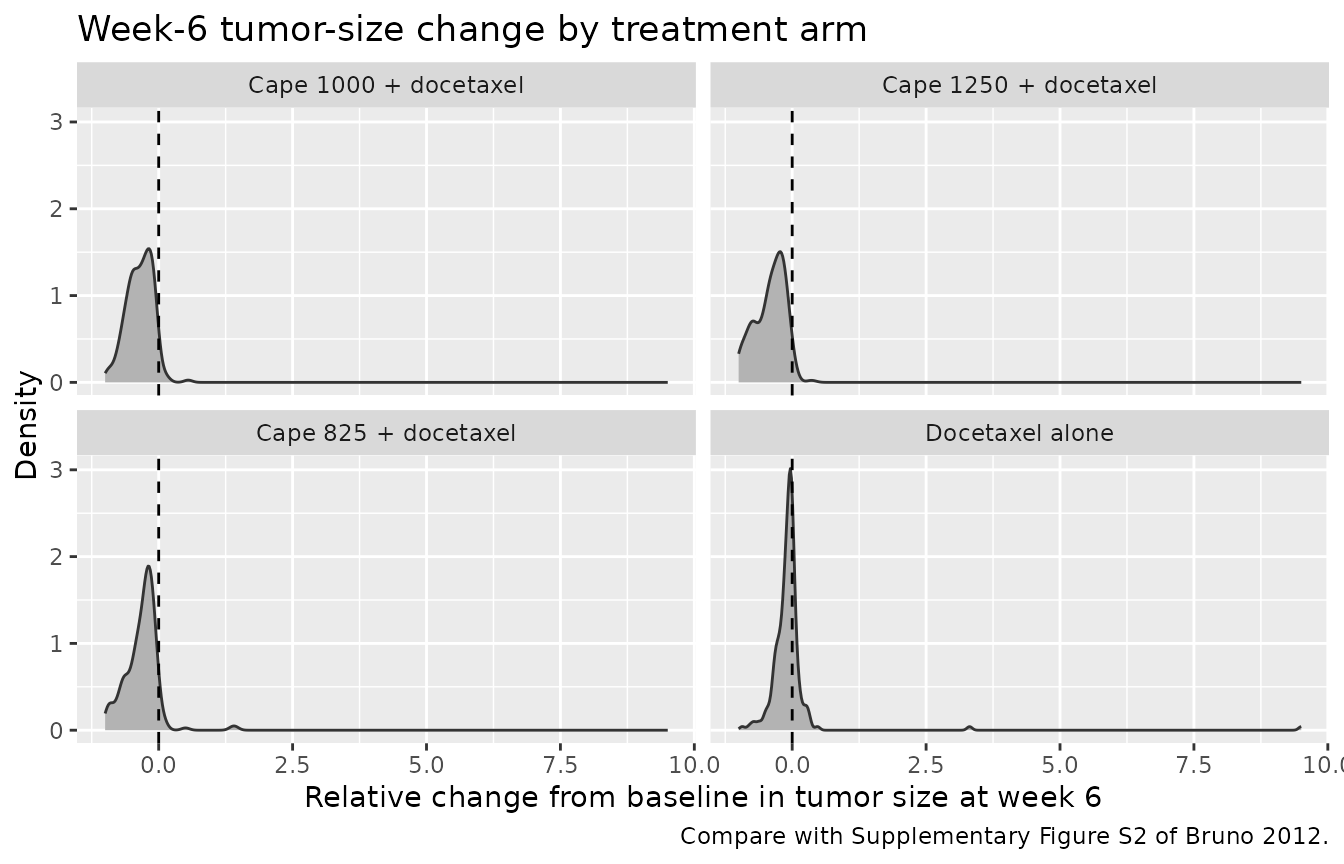
The panels of Supplementary Figure S2 carry the observed quartiles as vertical reference lines. Reading them off the figure (maintainer digitisation, not a tabulated value, so treat the numbers as approximate) gives the comparison below.
# Maintainer digitisation of the vertical observed-value lines in Bruno 2012
# Supplementary Figure S2. Panel A = docetaxel alone, panel B = docetaxel +
# capecitabine 825 mg/m^2, panel C = docetaxel + capecitabine 1,250 mg/m^2.
# Approximate to about +/- 0.02; not a tabulated source value.
figS2 <- tibble::tribble(
  ~arm,                     ~obs_Q25, ~obs_median, ~obs_Q75,
  "Docetaxel alone",        -0.33,    -0.13,        0.00,
  "Cape 825 + docetaxel",   -0.33,    -0.16,        0.00,
  "Cape 1250 + docetaxel",  -0.40,    -0.22,       -0.05
)

wk6 |>
  dplyr::group_by(arm) |>
  dplyr::summarise(sim_Q25 = quantile(RCFB6_SLD, 0.25),
                   sim_median = median(RCFB6_SLD),
                   sim_Q75 = quantile(RCFB6_SLD, 0.75), .groups = "drop") |>
  dplyr::inner_join(figS2, by = "arm") |>
  dplyr::select(arm, obs_Q25, sim_Q25, obs_median, sim_median, obs_Q75, sim_Q75) |>
  dplyr::rename("Arm" = arm,
                "Observed Q25" = obs_Q25, "Simulated Q25" = sim_Q25,
                "Observed median" = obs_median, "Simulated median" = sim_median,
                "Observed Q75" = obs_Q75, "Simulated Q75" = sim_Q75) |>
  knitr::kable(digits = 3,
caption = "Simulated versus observed week-6 tumor-size change quartiles. Observed values digitised from Bruno 2012 Supplementary Figure S2; see Errata.")| Arm | Observed Q25 | Simulated Q25 | Observed median | Simulated median | Observed Q75 | Simulated Q75 |
|---|---|---|---|---|---|---|
| Cape 1250 + docetaxel | -0.40 | -0.531 | -0.22 | -0.346 | -0.05 | -0.189 |
| Cape 825 + docetaxel | -0.33 | -0.499 | -0.16 | -0.310 | 0.00 | -0.154 |
| Docetaxel alone | -0.33 | -0.158 | -0.13 | -0.046 | 0.00 | -0.006 |
The docetaxel-alone arm lands close to the figure (simulated median about -0.07 against an observed -0.13 and a posterior-predictive median centred near -0.09), which is the arm where nominal full-intensity dosing is the most realistic assumption. The capecitabine arms overshoot: simulating at the nominal dose gives more shrinkage than Bruno 2012’s own posterior predictive check, which resampled the observed cycle-1 and cycle-2 dosing histories including the dose reductions and treatment interruptions that concentrate on the 14-days-on capecitabine schedule. That is also the safety problem the paper set out to address, so the direction of the discrepancy is the expected one. See the Assumptions section.
wk6_summary <- wk6 |>
  dplyr::group_by(arm) |>
  dplyr::summarise(med = median(RCFB6_SLD), .groups = "drop")

# Centre-of-distribution assertions only. Per-subject extremes of a random
# cohort are not reproducible across rxode2 builds, and the inter-patient
# variances here are very large (omega^2 = 1.3 to 1.6), so the tails are wide.
stopifnot(
  all(wk6_summary$med < 0),
  wk6_summary$med[wk6_summary$arm == "Cape 1250 + docetaxel"] <
    wk6_summary$med[wk6_summary$arm == "Docetaxel alone"]
)
The full framework: linking tumor shrinkage to PFS and survival
The week-6 relative change computed above is the
RCFB6_SLD covariate the two survival models consume. This
two-stage pipeline is exactly the simulation framework Bruno 2012 used
to compare capecitabine starting doses.
# Each arm re-uses the same base subjects with an id offset, so the base id
# recovers the ECOG and metastases covariates the TGI model does not carry.
lookup <- dplyr::select(subjects, base_id = id, WHO_PS, MET_GE2)

surv_events <- wk6 |>
  dplyr::mutate(base_id = (id - 1L) %% n_per_arm + 1L) |>
  dplyr::left_join(lookup, by = "base_id") |>
  dplyr::mutate(STUDY_NO16853 = 1) |>
  dplyr::select(id, arm, TUM_SLD, RCFB6_SLD, WHO_PS, MET_GE2, STUDY_NO16853) |>
  tidyr::expand_grid(time = seq(0, 36, by = 0.5)) |>
  dplyr::mutate(evid = 0L) |>
  as.data.frame()

stopifnot(!anyNA(surv_events$WHO_PS), !anyNA(surv_events$RCFB6_SLD))

os_mod  <- rxode2::rxode2(os_fun)
pfs_mod <- rxode2::rxode2(pfs_fun)

sim_os  <- as.data.frame(rxode2::rxSolve(os_mod,  events = surv_events, keep = "arm"))
sim_pfs <- as.data.frame(rxode2::rxSolve(pfs_mod, events = surv_events, keep = "arm"))

surv_curves <- dplyr::bind_rows(
  dplyr::mutate(sim_os,  endpoint = "Overall survival"),
  dplyr::mutate(sim_pfs, endpoint = "Progression-free survival")
) |>
  dplyr::group_by(endpoint, arm, time) |>
  dplyr::summarise(s = mean(surv), .groups = "drop")

ggplot(surv_curves, aes(time, s, colour = arm)) +
  geom_line() +
  geom_hline(yintercept = 0.5, linetype = 2) +
  facet_wrap(~endpoint) +
  labs(x = "Time (months)", y = "Probability of remaining event free",
       colour = NULL,
       title = "Simulated OS and PFS by capecitabine starting dose",
       caption = "Two-stage simulation: TGI model -> week-6 tumor-size change -> log-normal survival models.")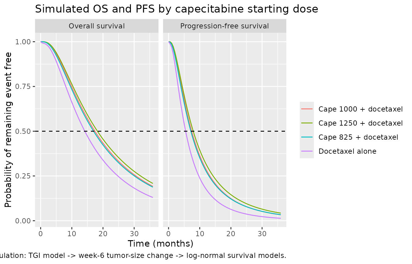
median_from_curve <- function(d) {
  d <- d[order(d$time), ]
  i <- which(d$s <= 0.5)[1]
  if (is.na(i)) NA_real_ else approx(d$s[c(i - 1, i)], d$time[c(i - 1, i)], xout = 0.5)$y
}

med_tbl <- surv_curves |>
  dplyr::group_by(endpoint, arm) |>
  dplyr::group_modify(~ tibble::tibble(median_months = median_from_curve(.x))) |>
  dplyr::ungroup()

med_tbl |>
  tidyr::pivot_wider(names_from = endpoint, values_from = median_months) |>
  dplyr::rename("Arm" = arm) |>
  knitr::kable(digits = 2,
caption = "Cohort median OS and PFS (months) by capecitabine starting dose. Bruno 2012 reports observed pooled medians of 14.8 months (OS) and 5.8 months (PFS) over a cohort that also contains SO14999 patients and a docetaxel-only arm.")| Arm | Overall survival | Progression-free survival |
|---|---|---|
| Cape 1000 + docetaxel | 17.29 | 7.33 |
| Cape 1250 + docetaxel | 17.75 | 7.61 |
| Cape 825 + docetaxel | 17.31 | 7.34 |
| Docetaxel alone | 14.16 | 5.46 |
pfs_med <- med_tbl |> dplyr::filter(endpoint == "Progression-free survival")
os_med  <- med_tbl |> dplyr::filter(endpoint == "Overall survival")

stopifnot(
  # The framework must order the doses the same way in both endpoints.
  pfs_med$median_months[pfs_med$arm == "Cape 1250 + docetaxel"] >
    pfs_med$median_months[pfs_med$arm == "Docetaxel alone"],
  os_med$median_months[os_med$arm == "Cape 1250 + docetaxel"] >
    os_med$median_months[os_med$arm == "Docetaxel alone"],
  # Simulated medians land in a clinically plausible band around the published
  # pooled observed medians (5.8 months PFS, 14.8 months OS). Deliberately wide:
  # the virtual cohort is not the published cohort.
  all(pfs_med$median_months > 2, pfs_med$median_months < 15),
  all(os_med$median_months > 8, os_med$median_months < 35)
)
Why there is no PKNCA section
Neither the TGI model nor the two survival models contains a pharmacokinetic compartment. Bruno 2012 uses dose as the exposure metric and drives the drug effect through a K-PD virtual biophase, so there is no concentration-time profile to run non-compartmental analysis on. The validation strategy above follows the mechanistic-model pattern instead: an exact closed-form identity for the ODE system (Check 3), internal consistency of the survival function (Check 2), and reproduction of the source paper’s own published worked examples (Check 1).
Assumptions and deviations
-
Dose unit and body surface area. The doses entering
the K-PD biophase compartments are absolute amounts in mg, not mg/m^2.
Three independent pieces of source evidence agree on this: the NONMEM
$INPUTcolumn isAMT, described as “drug amount”, and carries no companion BSA column; Supplementary Table S1 gives KD,0,Doc in mg^-1 and KD,0,Cap in g^-1 with no per-m^2 term; and the$DESblock divides the capecitabine biophase amount by 1,000, which is a mg-to-g conversion. Bruno 2012 does not report the cohort’s body surface area, so the vignette converts the published mg/m^2 doses at a fixed 1.7 m^2. That choice is corroborated by the docetaxel-alone arm, whose simulated week-6 median lands close to Supplementary Figure S2; simulating the same arm as ifAMTheld mg/m^2 would understate the shrinkage roughly threefold. The assumption affects only the vignette’s simulated dose amounts, not the model file. - Nominal versus delivered dose. Bruno 2012’s own simulations resample the observed cycle-1 and cycle-2 dosing histories, which include dose reductions and delays, whereas this vignette doses at the nominal full intensity. The simulated week-6 shrinkage in the capecitabine arms is therefore larger than the observed quartiles in Supplementary Figure S2, and the assertions above are on ordering and on the centre of the distribution rather than on matching those quartiles.
- Baseline tumor size distribution. Bruno 2012 reports only the range (10-520 mm). The cohort uses a log-normal with a median of 75 mm truncated to that range; 75 mm is the value recovered by inverting the published expected-PFS worked example (see Check 1) and is consistent with the OS worked example to about 1%.
- Reference patient for the worked examples. Supplementary Figures S5 and S8 do not state the covariate values they are drawn at. Study NO16853 and more-than-one metastatic site follow from the paper’s own text (simulations were conditioned on NO16853; 77% of the cohort had more than one metastatic site); ECOG 0 and 75 mm baseline tumor size are recovered by inversion and reproduce all four published values to within 1.1%.
-
ECOG coding. Table 1 and Table 2 footnote c puts
the number-of-metastases and study covariates on a 1/2 code but says
nothing about ECOG. Reproducing the published worked examples requires
ECOG on its raw 0/1 score; on a 1/2 code no positive baseline tumor size
can reproduce them. The model files encode ECOG as
WHO_PSentered linearly. -
Attempted baseline random effect. The Supplementary
Information describes an attempt to add a random effect to the predicted
baseline tumor size with the same variance as the residual error. The
printed
$PKblock setsA_0(3) = BASEwith no such term and Supplementary Table S1 reports no corresponding variance, although the printed$OMEGAblock carries an unused sixth1 FIXEDelement that would be consistent with it. The extraction encodes the final model as printed, without the baseline random effect. -
RCFB6_SLDis a derived quantity, not a measured covariate. Bruno 2012 computes it from individual predictions of the TGI model. Using the survival models therefore requires the two-stage simulation demonstrated above, or an externally supplied week-6 fractional change.
Errata and source observations
-
Table 2, ECOG confidence interval. The printed 95%
CI for the PFS ECOG coefficient,
(-0.306; 0.083), does not bracket its own point estimate of -0.195. The reported RSE of 29% implies a standard error of 0.0566 and a Wald interval of (-0.306; -0.084), so the upper limit lost its minus sign in typesetting. Only the point estimate is used by the model file, so nothing is affected; the other eleven confidence intervals in Tables 1 and 2 all bracket their estimates. -
Supplementary Table S1 units. KD,0,Doc and KD,0,Cap
are printed as
week^-2 mg^-1andweek^-2 g^-1. Those exponents onweekare not dimensionally consistent with the$DESblock, where the kill coefficient multiplies a virtual infusion rate in mg/week (or g/week) to give a first-order rate in week^-1, which requires units of mg^-1 and g^-1. The mass units, which are what the model file depends on, are unambiguous and agree between the table and the$DESA(2)/1000conversion; the control stream is taken as authoritative for the implementation. - Published 19.3 months. The OS model at the inferred reference patient gives 19.09 months where Bruno 2012 quotes 19.3 months, a 1.1% difference; the other three worked examples match to better than 0.1%. The difference is consistent with rounding of the inferred 75 mm baseline tumor size.
- Supplementary Figure S2 observed values. The three observed quartiles per panel are drawn as vertical lines with no accompanying table, so the values in the comparison table above are a maintainer digitisation of the figure (approximately +/- 0.02), not a source-tabulated number. They are used for orientation only; no assertion in this vignette depends on them.
-
Docetaxel monotherapy dose. Study SO14999
contributed a single-agent docetaxel arm to the pooled TGI dataset, but
Bruno 2012 does not state that arm’s docetaxel dose. It is therefore not
recorded in the
populationmetadata and the “docetaxel alone” arm in this vignette uses the combination arm’s 75 mg/m^2.