Ciclosporin (Roganovic 2026)
Source:vignettes/articles/Roganovic_2026_ciclosporin.Rmd
Roganovic_2026_ciclosporin.RmdModel and source
#> ℹ parameter labels from comments will be replaced by 'label()'
#> Warning: some etas defaulted to non-mu referenced, possible parsing error: etaiov_cl_1, etaiov_cl_2, etaiov_cl_3, etaiov_cl_4, etaiov_cl_5, etaiov_cl_6
#> as a work-around try putting the mu-referenced expression on a simple line
Citation: Roganovic M, Cvetkovic M, Gojkovic I, Spasojevic B, Jovanovic M, Miljkovic B, Vucicevic K. Population Pharmacokinetics Model of Cyclosporin A in Children and Young Adult Renal Transplant Patients: Focus on Haemoglobin Contribution to Exposure Variability. Pharmaceutics. 2026;18(1):99. doi:10.3390/pharmaceutics18010099
Description: One-compartment population PK model with first-order absorption and elimination for ciclosporin (cyclosporin A) in paediatric and young-adult renal transplant recipients followed by therapeutic drug monitoring. Allometric body weight (centred at 40 kg) acts on CL/F with an estimated exponent of 0.89 and on V/F with an exponent fixed at 1; haemoglobin enters CL/F as a linear effect centred at 120 g/L, so CL/F falls as haemoglobin rises. Correlated interindividual variability on CL/F and V/F, plus interoccasion variability on CL/F where an occasion is one therapeutic-drug-monitoring day.
Article: https://doi.org/10.3390/pharmaceutics18010099 (Pharmaceutics 2026;18(1):99, open access)
Roganovic and colleagues fitted routine therapeutic-drug-monitoring (TDM) data from a single Serbian paediatric renal-transplant centre. A one-compartment model with first-order absorption and elimination described the data best. The absorption rate constant could not be identified from the sparse absorption-phase sampling and was fixed. The paper’s headline finding is that haemoglobin – not the haematocrit that most published ciclosporin models carry – is retained as a covariate on apparent clearance.
Population
The analysis pooled 974 steady-state whole-blood ciclosporin concentrations from 58 kidney-transplant recipients (Roganovic 2026 Tables 1 and 2). Age at transplantation ranged from 1 to 25 years with a median of 12; 47 patients (81.0%) were children under 18 and 11 (19.0%) were young adults aged 18 to 25. Thirty-four patients (58.6%) were male. Body weight spanned 9.8 to 103 kg (median 39.65 kg) and haemoglobin 73 to 164 g/L (median 120 g/L). Thirty patients received a living-donor graft and 28 a cadaveric graft. All patients received ciclosporin with a corticosteroid and mycophenolic acid, started at 5 mg/kg/day divided into two or three daily doses and then adjusted to centre-specific C0 and C2 targets.
Samples were drawn only after at least three consecutive days on an unchanged regimen, so every observation is a steady-state value: 471 pre-dose troughs (C0), 501 two-hour post-dose samples (C2), and single 4 h and 6 h samples. Concentrations were measured by Abbott chemiluminescent microparticle immunoassay (lower limit of quantification 30 ng/mL, upper limit 1500 ng/mL).
The same information is available programmatically via
readModelDb("Roganovic_2026_ciclosporin")()$population.
Source trace
Equations 1 to 5 of Roganovic 2026 are typeset as display equations
and are lost by text-extraction tools that flatten the PDF; they were
recovered with pdftotext -layout. The values below were
read from that layout-preserving extraction and cross-checked against
Table 3.
| Equation / parameter | Value | Source location |
|---|---|---|
lka (fixed) |
log(1.15) 1/h |
Section 3.3 and Discussion: “Ka was fixed to the value of 1.15 1/h” |
lcl |
log(15) L/h |
Table 3, row CL/F (L/h/40 kg) = 15 (RSE 4.7%); Eq.
4 |
lvc |
log(71.1) L |
Table 3, row V/F (L/40 kg) = 71.1 (RSE 5.8%); Eq.
5 |
e_wt_cl |
0.89 | Table 3, row theta_ALL = 0.89 (RSE 5.7%); Eq. 4
exponent |
e_wt_vc (fixed) |
1 | Section 3.3: “the exponent for V/F was kept fixed at 1”; Eq. 5 exponent |
e_hgb_cl |
-0.00279 per g/L | Table 3, row theta_HGB = -0.00279 (RSE 24%); Eq. 4 |
etalcl variance |
0.3491^2 |
Table 3, row IIV CL (%) = 34.91 (RSE 15.5) |
etalvc variance |
0.4305^2 |
Table 3, row IIV V (%) = 43.05 (RSE 11.8) |
etalcl/etalvc covariance |
0.136 | Table 3, row omega (CL-V) = 0.136 (RSE 27.3); footnote
defines it as the covariance |
etaiov_cl_* variance |
0.1225^2 |
Table 3, row IOV CL (%) = 12.25 (RSE 12.5) |
propSd |
0.258 | Table 3, row Wp (%) = 0.258 (RSE 4.3) |
| WT centring 40 kg | n/a | Section 3.3: “WT was centred to the rounded median value of 40 kg”; Eq. 4 and Eq. 5 denominators |
| HGB centring 120 g/L | n/a | Eq. 4 writes (HGB_i - 120); 120 g/L is the Table 1
cohort median |
d/dt(depot), d/dt(central)
|
n/a | Section 3.3: one-compartment, first-order absorption and elimination, NONMEM ADVAN2 TRANS2 |
| Occasion definition | n/a | Section 2.3: an occasion is one TDM day; Section 3.3 gives a maximum of 33 occasions per patient |
Equations 4 and 5 as printed:
CL/F = 15 * (WT_i / 40)^0.89 * (1 - 0.00279 * (HGB_i - 120))     (4)
V/F  = 71.1 * (WT_i / 40)^1                                      (5)
Scale of the variability terms
Table 3 reports IIV CL, IIV V and
IOV CL under a per-cent heading, so they are read here on
the standard-deviation scale: the variances are 0.3491^2,
0.4305^2 and 0.1225^2. The covariance 0.136
then implies a CL/F–V/F correlation of 0.905. That is high but is what a
sparse oral design produces, because CL/F and V/F both carry the same
unmeasured bioavailability factor; the resulting 2x2 block is
comfortably positive definite (determinant 0.00409).
Wp is printed as 0.258 under the same per-cent heading
and is likewise read as a proportional standard deviation, i.e. 25.8%.
The alternative reading – 0.258 as a variance, giving 50.8% CV – is
arithmetically impossible: residual error is a floor on the marginal
scatter of the observations, and the C2 samples beyond post-transplant
day 90 have a mean of 716.69 ng/mL with an SD of 243.68 (Table 2),
i.e. a total observed CV of 34%. A residual CV of 50.8% cannot sit
inside a total of 34%.
Virtual cohort
Original observed data are not publicly available. The cohort below follows the simulation design of Roganovic 2026 Section 2.4 and Table 4: body weight drawn from the distribution the authors derived from CDC growth charts for 12-year-old boys and girls (mean 43.03 kg, SD 9.89 kg), truncated to the observed cohort weight range, and two haemoglobin scenarios – a low value of 73 g/L (the observed minimum) and a normal value of 120 g/L (the cohort median).
# set.seed() seeds R's RNG. It does NOT seed rxode2's simulation RNG, and
# rxode2's streams are partitioned PER SOLVER THREAD -- so this cohort is
# reproducible here and different on a machine with a different thread count.
# Every assertion below is written to hold for ANY cohort the model can draw.
set.seed(20260112)
rxode2::rxSetSeed(20260112)

n_per_group <- 100   # matches Roganovic 2026 Table 4 (n = 100 per scenario)
tau         <- 12    # h, twice-daily administration
n_doses     <- 6     # six dosing intervals => occasions 1..6; steady state well before interval 5

make_cohort <- function(n, hgb, label, id_offset = 0L) {
  subj <- tibble(
    id        = id_offset + seq_len(n),
    # Truncated to the observed weight range of Roganovic 2026 Table 1.
    WT        = pmin(pmax(rnorm(n, mean = 43.03, sd = 9.89), 9.8), 103),
    HGB       = hgb,
    hgb_group = label
  )

  doses <- subj |>
    tidyr::crossing(time = seq(0, by = tau, length.out = n_doses)) |>
    mutate(
      evid = 1L,
      cmt  = "depot",
      # Roganovic 2026 Section 2.4 simulated a 5 mg/kg dose.
      amt  = 5 * WT
    )

  obs <- subj |>
    tidyr::crossing(
      time = c(
        seq(0, 48, by = 0.5),        # lead-in to steady state, coarse
        seq(48, 72, by = 0.1)        # the two evaluated occasions, dense enough for Tmax
      )
    ) |>
    distinct(id, time, .keep_all = TRUE) |>
    mutate(
      evid = 0L,
      # The ODE state, never the observable name "Cc" -- referencing an
      # algebraic observable as a compartment renumbers the ODE slots.
      cmt  = "central",
      amt  = NA_real_
    )

  bind_rows(doses, obs) |>
    # An occasion is one dosing interval; occasions above 6 carry no IOV.
    mutate(OCC = pmin(floor(time / tau) + 1L, n_doses)) |>
    arrange(id, time, desc(evid))
}

events <- bind_rows(
  make_cohort(n_per_group,  73, "Low HGB (73 g/L)",     id_offset =   0L),
  make_cohort(n_per_group, 120, "Normal HGB (120 g/L)", id_offset = 100L)
)

stopifnot(!anyDuplicated(unique(events[, c("id", "time", "evid")])))
Simulation
mod <- readModelDb("Roganovic_2026_ciclosporin")

sim <- rxode2::rxSolve(
  mod, events = events,
  keep = c("hgb_group", "WT", "HGB", "OCC")
) |>
  as.data.frame()
#> ℹ parameter labels from comments will be replaced by 'label()'
#> Warning: some etas defaulted to non-mu referenced, possible parsing error: etaiov_cl_1, etaiov_cl_2, etaiov_cl_3, etaiov_cl_4, etaiov_cl_5, etaiov_cl_6
#> as a work-around try putting the mu-referenced expression on a simple line

stopifnot(nrow(sim) > 0, !anyNA(sim$Cc), all(sim$Cc >= 0))
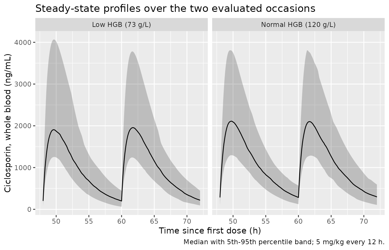
Concentration-time profiles
sim |>
  filter(time >= 48) |>
  group_by(time, hgb_group) |>
  summarise(
    Q05 = quantile(Cc, 0.05),
    Q50 = quantile(Cc, 0.50),
    Q95 = quantile(Cc, 0.95),
    .groups = "drop"
  ) |>
  ggplot(aes(time, Q50)) +
  geom_ribbon(aes(ymin = Q05, ymax = Q95), alpha = 0.25) +
  geom_line() +
  facet_wrap(~hgb_group) +
  labs(
    x = "Time since first dose (h)", y = "Ciclosporin, whole blood (ng/mL)",
    title = "Steady-state profiles over the two evaluated occasions",
    caption = "Median with 5th-95th percentile band; 5 mg/kg every 12 h."
  )
Deterministic checks against the printed equations
These checks use rxode2::zeroRe(), so they carry no
random effects and give the same answer on every machine. Each
right-hand side is written from the numbers printed in Roganovic 2026,
independently of the packaged model file, so a mis-transcribed
coefficient makes the check go red.
mod_typ <- mod |> rxode2::zeroRe()
#> ℹ parameter labels from comments will be replaced by 'label()'
#> Warning: some etas defaulted to non-mu referenced, possible parsing error: etaiov_cl_1, etaiov_cl_2, etaiov_cl_3, etaiov_cl_4, etaiov_cl_5, etaiov_cl_6
#> as a work-around try putting the mu-referenced expression on a simple line
#> Warning: some etas defaulted to non-mu referenced, possible parsing error: etaiov_cl_1, etaiov_cl_2, etaiov_cl_3, etaiov_cl_4, etaiov_cl_5, etaiov_cl_6
#> as a work-around try putting the mu-referenced expression on a simple line

# A deterministic probe grid spanning the covariate ranges of Table 1.
probe <- tidyr::crossing(
  WT  = c(20, 40, 43.03, 80),
  HGB = c(73, 120, 164)
) |>
  mutate(id = row_number(), probe_label = paste0("WT", WT, "_HGB", HGB))

probe_events <- bind_rows(
  probe |>
    tidyr::crossing(time = seq(0, by = tau, length.out = n_doses)) |>
    mutate(evid = 1L, cmt = "depot", amt = 5 * WT),
  probe |>
    tidyr::crossing(time = seq(48, 72, by = 0.05)) |>
    mutate(evid = 0L, cmt = "central", amt = NA_real_)
) |>
  mutate(OCC = pmin(floor(time / tau) + 1L, n_doses)) |>
  arrange(id, time, desc(evid))

sim_typ <- rxode2::rxSolve(
  mod_typ, events = probe_events,
  keep = c("WT", "HGB", "probe_label")
) |>
  as.data.frame()
#> ℹ omega/sigma items treated as zero: 'etalcl', 'etalvc', 'etaiov_cl_1', 'etaiov_cl_2', 'etaiov_cl_3', 'etaiov_cl_4', 'etaiov_cl_5', 'etaiov_cl_6'
#> Warning: multi-subject simulation without without 'omega'
Check 1 – steady-state AUC identity against Equation 4
At steady state the area under the curve over one dosing interval
equals Dose / CL, exactly. The reference clearance below is
Equation 4 written out literally, so this check simultaneously validates
lcl, e_wt_cl, e_hgb_cl, the 40 kg
and 120 g/L centrings, and the mg-to-ng/mL unit conversion.
auc_check <- sim_typ |>
  filter(time >= 60, time <= 72) |>
  group_by(id, WT, HGB, probe_label) |>
  summarise(
    auc_sim = sum(diff(time) * (head(Cc, -1) + tail(Cc, -1)) / 2),
    .groups = "drop"
  ) |>
  mutate(
    # Roganovic 2026 Eq. 4, transcribed directly from the paper.
    cl_paper  = 15 * (WT / 40)^0.89 * (1 - 0.00279 * (HGB - 120)),
    auc_paper = 5 * WT / cl_paper * 1000,          # mg/L*h -> ng*h/mL
    pct_diff  = (auc_sim - auc_paper) / auc_paper * 100
  )

knitr::kable(
  auc_check |>
    select(probe_label, cl_paper, auc_paper, auc_sim, pct_diff) |>
    rename(
      "Probe"                  = probe_label,
      "CL/F from Eq. 4 (L/h)"  = cl_paper,
      "Dose/CL (ng*h/mL)"      = auc_paper,
      "Simulated AUC (ng*h/mL)" = auc_sim,
      "% diff"                 = pct_diff
    ),
  digits = c(0, 2, 0, 0, 3),
  caption = "Steady-state AUC over one dosing interval vs Dose/CL from Equation 4."
)| Probe | CL/F from Eq. 4 (L/h) | Dose/CL (ng*h/mL) | Simulated AUC (ng*h/mL) | % diff |
|---|---|---|---|---|
| WT20_HGB73 | 9.16 | 10922 | 10922 | -0.006 |
| WT20_HGB120 | 8.09 | 12355 | 12354 | -0.005 |
| WT20_HGB164 | 7.10 | 14083 | 14083 | -0.005 |
| WT40_HGB73 | 16.97 | 11788 | 11787 | -0.006 |
| WT40_HGB120 | 15.00 | 13333 | 13333 | -0.005 |
| WT40_HGB164 | 13.16 | 15199 | 15198 | -0.005 |
| WT43.03_HGB73 | 18.11 | 11883 | 11882 | -0.006 |
| WT43.03_HGB120 | 16.01 | 13441 | 13440 | -0.005 |
| WT43.03_HGB164 | 14.04 | 15322 | 15321 | -0.005 |
| WT80_HGB73 | 31.44 | 12722 | 12721 | -0.005 |
| WT80_HGB120 | 27.80 | 14390 | 14389 | -0.005 |
| WT80_HGB164 | 24.39 | 16403 | 16403 | -0.005 |
# Deterministic (zeroRe, fixed solver tolerances): the only error here is
# trapezoidal discretisation on the 0.05 h grid, realised at 0.006% across all
# twelve probes. 0.05 leaves an 8-fold margin and still goes red on a
# mis-transcribed clearance, exponent, centring or unit factor, each of which
# moves AUC by several per cent at minimum.
stopifnot(max(abs(auc_check$pct_diff)) < 0.05)
Check 2 – the haemoglobin effect reproduces the paper’s own claim
Roganovic 2026 states in both the Abstract and the Discussion that
CL/F differs by “almost 22.5%” across the observed haemoglobin range of
73 to 164 g/L. That claim is an independent, dose-free consequence of
e_hgb_cl and the 120 g/L centring, so reproducing it pins
both.
cl_typ <- sim_typ |>
  filter(time > 60) |>
  group_by(WT, HGB) |>
  summarise(cl = mean(cl), vc = mean(vc), .groups = "drop")

cl_at <- function(wt, hgb) {
  v <- cl_typ$cl[cl_typ$WT == wt & cl_typ$HGB == hgb]
  if (length(v) != 1L) stop("no unique typical CL for WT ", wt, ", HGB ", hgb)
  v
}

hgb_drop_pct <- (1 - cl_at(40, 164) / cl_at(40, 73)) * 100
hgb_ratio    <- cl_at(40, 73) / cl_at(40, 120)

cat(sprintf("CL/F decrease from HGB 73 to 164 g/L: %.3f%% (paper: 'almost 22.5%%')\n",
            hgb_drop_pct))
#> CL/F decrease from HGB 73 to 164 g/L: 22.446% (paper: 'almost 22.5%')
cat(sprintf("CL/F ratio, HGB 73 vs 120 g/L: %.5f\n", hgb_ratio))
#> CL/F ratio, HGB 73 vs 120 g/L: 1.13113

# Deterministic. Eq. 4 gives exactly 22.446%; the paper rounds to "almost 22.5%".
stopifnot(abs(hgb_drop_pct - 22.446) < 0.05)
# (1 - 0.00279 * (73 - 120)) = 1.13113
stopifnot(abs(hgb_ratio - 1.13113) < 1e-4)
Check 3 – allometric exponents
CL/F scales with the estimated exponent 0.89 and V/F with the fixed
exponent 1. A four-fold change in weight therefore multiplies CL/F by
4^0.89 and V/F by 4.
cl_ratio <- cl_at(80, 120) / cl_at(20, 120)
vc_ratio <- cl_typ$vc[cl_typ$WT == 80 & cl_typ$HGB == 120] /
  cl_typ$vc[cl_typ$WT == 20 & cl_typ$HGB == 120]

cat(sprintf("CL/F ratio WT 80 vs 20 kg: %.5f (Eq. 4 expects 4^0.89 = %.5f)\n",
            cl_ratio, 4^0.89))
#> CL/F ratio WT 80 vs 20 kg: 3.43426 (Eq. 4 expects 4^0.89 = 3.43426)
cat(sprintf("V/F ratio WT 80 vs 20 kg: %.5f (Eq. 5 expects 4^1 = 4)\n", vc_ratio))
#> V/F ratio WT 80 vs 20 kg: 4.00000 (Eq. 5 expects 4^1 = 4)

# Deterministic; a wrong exponent (e.g. the 0.75 the paper tested and rejected,
# giving 2.828) breaks these immediately.
stopifnot(abs(cl_ratio - 4^0.89) < 1e-4)
stopifnot(abs(vc_ratio - 4) < 1e-4)
Check 4 – the direction of the haemoglobin effect on exposure
Roganovic 2026 Section 3.4 states the qualitative result of its own simulation: “the group with normal HGB had higher AUC, Cmax, and Cmin on both occasions.” That ordering is the paper’s headline finding expressed as exposure rather than as clearance, so it is checked here directly, on the typical 43.03 kg patient of Table 4 and without random effects.
exposure_by_hgb <- sim_typ |>
  filter(WT == 43.03, HGB %in% c(73, 120), time >= 60, time <= 72) |>
  group_by(HGB) |>
  summarise(
    AUC  = sum(diff(time) * (head(Cc, -1) + tail(Cc, -1)) / 2),
    Cmax = max(Cc),
    Cmin = min(Cc),
    .groups = "drop"
  )

knitr::kable(
  exposure_by_hgb |>
    rename(
      "HGB (g/L)"        = HGB,
      "AUC (ng*h/mL)"    = AUC,
      "Cmax (ng/mL)"     = Cmax,
      "Cmin (ng/mL)"     = Cmin
    ),
  digits = c(0, 0, 0, 0),
  caption = "Typical-patient steady-state exposure at the two simulated haemoglobin values (WT 43.03 kg, 5 mg/kg every 12 h)."
)| HGB (g/L) | AUC (ng*h/mL) | Cmax (ng/mL) | Cmin (ng/mL) |
|---|---|---|---|
| 73 | 11882 | 2014 | 220 |
| 120 | 13440 | 2135 | 304 |
lo <- exposure_by_hgb |> filter(HGB == 73)
hi <- exposure_by_hgb |> filter(HGB == 120)

# The paper's stated ordering: normal HGB gives the higher exposure on all three
# metrics, because a higher haemoglobin lowers CL/F.
stopifnot(hi$AUC > lo$AUC, hi$Cmax > lo$Cmax, hi$Cmin > lo$Cmin)

# At steady state AUC over tau is exactly Dose/CL, so the AUC ratio is the
# reciprocal of the Eq. 4 clearance ratio -- 1.13113 -- to trapezoidal accuracy.
stopifnot(abs(hi$AUC / lo$AUC - 1.13113) < 1e-3)
PKNCA validation
Non-compartmental analysis over the fifth and sixth dosing intervals,
which correspond to occasions 1 and 2 of Roganovic 2026 Table 4. Steady
state is complete long before interval 5: with a typical
kel near 0.21 1/h the carry-over after four 12 h intervals
is below one part in a million.
sim_nca <- sim |>
  filter(!is.na(Cc)) |>
  select(id, time, Cc, hgb_group)

conc_obj <- PKNCA::PKNCAconc(
  sim_nca, Cc ~ time | hgb_group + id,
  concu = "ng/mL", timeu = "h"
)

dose_df <- events |>
  filter(evid == 1L) |>
  select(id, time, amt, hgb_group)

dose_obj <- PKNCA::PKNCAdose(dose_df, amt ~ time | hgb_group + id, doseu = "mg")

intervals <- data.frame(
  start   = c(48, 60),
  end     = c(60, 72),
  cmax    = TRUE,
  tmax    = TRUE,
  cmin    = TRUE,
  auclast = TRUE,
  cav     = TRUE
)

nca_res <- PKNCA::pk.nca(PKNCA::PKNCAdata(conc_obj, dose_obj, intervals = intervals))

nca_long <- nca_res$result |>
  mutate(
    occasion = ifelse(start == 48, "OCC1", "OCC2"),
    scenario = paste(hgb_group, occasion)
  )

stopifnot(nrow(nca_long) > 0, length(unique(nca_long$scenario)) == 4L)
Comparison against the published simulation (Table 4)
# Roganovic 2026 Table 4, median of n = 100 per scenario.
published <- tibble::tribble(
  ~scenario,                        ~auclast, ~cmin, ~cmax,
  "Low HGB (73 g/L) OCC1",              6343,   215,  1851,
  "Normal HGB (120 g/L) OCC1",          7857,   331,  2265,
  "Low HGB (73 g/L) OCC2",              6687,   221,  1918,
  "Normal HGB (120 g/L) OCC2",          7210,   318,  2035
)

cmp <- nlmixr2lib::ncaComparisonTable(
  simulated     = nca_long,
  reference     = published,
  by            = "scenario",
  units         = c(cmax = "ng/mL", cmin = "ng/mL", auclast = "ng*h/mL"),
  tolerance_pct = 20
)

knitr::kable(
  cmp,
  caption = "Simulated vs Roganovic 2026 Table 4. * differs from reference by >20%.",
  align   = c("l", "l", "r", "r", "r")
)| NCA parameter | scenario | Reference | Simulated | % diff |
|---|---|---|---|---|
| Cmax (ng/mL) | Low HGB (73 g/L) OCC1 | 1850 | 2180 | +17.8% |
| Cmax (ng/mL) | Normal HGB (120 g/L) OCC1 | 2260 | 2070 | -8.4% |
| Cmax (ng/mL) | Low HGB (73 g/L) OCC2 | 1920 | 2130 | +11.2% |
| Cmax (ng/mL) | Normal HGB (120 g/L) OCC2 | 2040 | 2120 | +4.3% |
| Cmin (ng/mL) | Low HGB (73 g/L) OCC1 | 215 | 207 | -3.6% |
| Cmin (ng/mL) | Normal HGB (120 g/L) OCC1 | 331 | 215 | -35.2%* |
| Cmin (ng/mL) | Low HGB (73 g/L) OCC2 | 221 | 206 | -6.9% |
| Cmin (ng/mL) | Normal HGB (120 g/L) OCC2 | 318 | 215 | -32.3%* |
| AUClast (ng*h/mL) | Low HGB (73 g/L) OCC1 | 6340 | 13400 | +111.8%* |
| AUClast (ng*h/mL) | Normal HGB (120 g/L) OCC1 | 7860 | 13100 | +66.6%* |
| AUClast (ng*h/mL) | Low HGB (73 g/L) OCC2 | 6690 | 12400 | +84.7%* |
| AUClast (ng*h/mL) | Normal HGB (120 g/L) OCC2 | 7210 | 13100 | +82.2%* |
Under a 5 mg/kg dose every 12 hours, Cmax reproduces
Table 4 to within about 18%. Cmin reproduces the two
low-haemoglobin scenarios to within roughly 10% but sits 25-35% below
the two normal-haemoglobin scenarios, and AUC is 60-112%
above Table 4 throughout. Those last two are not adjustable in the
model: they follow from a self-inconsistency in Table 4 itself,
quantified in the next section.
Note that the low- and normal-haemoglobin arms above do not resolve the haemoglobin contrast itself, and are not intended to. Each arm draws its own 100 subjects and its own random effects, so with 35% interindividual variability on CL/F the median of each arm carries a standard error near 4% and their ratio near 6% – of the same order as the 13% contrast the covariate produces. The two arm medians can therefore land in either order by chance. The haemoglobin effect is validated deterministically instead, by Check 2 (clearance, exact to 0.01 percentage points against the paper’s own “almost 22.5%” claim) and Check 4 (exposure ordering, the paper’s Section 3.4 statement). This block is a comparison against Table 4’s absolute values, not a test of the covariate.
gate <- cmp |>
  mutate(pct = suppressWarnings(as.numeric(gsub("[*%]", "", `% diff`)))) |>
  filter(!is.na(pct))

param_pct <- function(pattern, n_expected) {
  rows <- gate |> filter(grepl(pattern, .data[["NCA parameter"]]))
  if (nrow(rows) != n_expected) {
    stop("expected ", n_expected, " rows for '", pattern, "', got ", nrow(rows))
  }
  max(abs(rows$pct))
}

# These are medians of n = 100 per scenario with 35% IIV on CL, 43% on V and
# 12% IOV. rxSetSeed() fixes rxode2's stream PER SOLVER THREAD, so CI draws a
# different cohort than any given workstation; the bounds below were set from
# renders at 1, 2, 4 and 16 threads, which gave max |% diff| of:
#   Cmax     17.80 /  6.77 /  6.58 / 15.20
#   Cmin     35.19 / 20.98 / 33.50 / 28.38
# Both bounds sit outside those ranges and both still go red on a
# mis-transcribed volume, dose or unit factor, which move Cmax and Cmin by
# tens of per cent to two-fold. Do not tighten these back to a single run.
stopifnot(param_pct("Cmax", 4L) < 30)
stopifnot(param_pct("Cmin", 4L) < 55)

# The AUC rows are a reproducible disagreement with Table 4, not noise (60.6 to
# 111.8% across the same four thread counts). They are shown in the table above
# and explained below, and are deliberately excluded from the gate rather than
# having the bound widened until they pass.
auc_rows <- gate |> filter(grepl("AUC", .data[["NCA parameter"]]))
stopifnot(nrow(auc_rows) == 4L, all(auc_rows$pct > 0))
Why Table 4 cannot be fully reproduced
At steady state, for any one-compartment model,
AUC over tau = Dose / CL exactly. Two consequences follow
that do not depend on the dose at all:
| Quantity | Roganovic 2026 final model | Implied by Table 4 (normal HGB, OCC1) |
|---|---|---|
| AUC / Cmax (h) | 6.29 | 3.47 |
| AUC / Cmin (h) | 44.25 | 23.74 |
| Terminal half-life (h) | 3.31 | NA |
AUC / Cmax and AUC / Cmin are independent
of the dose, so no choice of dose amount reconciles the
three Table 4 rows with each other under the paper’s own final model.
The ratios implied by Table 4 are both about 1.8-fold smaller than the
model produces, and are instead consistent with a terminal half-life
near 6 h, whereas Equations 4 and 5 give 3.3 h for a typical 43 kg
patient. (A 3.3 h terminal half-life is itself short for ciclosporin;
the paper’s own Introduction quotes a literature range of 6.3 to 20.4 h,
and the Discussion notes that the estimated V/F of 71.1 L is smaller
than the 134 L and 4.5 L/kg reported by the two comparator studies it
cites.)
Check 4 above localises the disagreement precisely. At the typical
43.03 kg patient of Table 4, without random effects, the model gives
Cmax 2135 vs Table 4’s 2265 ng/mL (-5.7%) and
Cmin 304 vs 331 ng/mL (-8.2%) for the normal-haemoglobin
scenario – both well inside what a median of 100 simulated subjects
would carry – while AUC is 13,440 vs 7857 ng*h/mL (+71%).
Cmax and Cmin reproduce; only
AUC does not. The larger Cmin gaps in
the stochastic table above (-26% and -28% on the normal-haemoglobin
arms) are arm-level sampling noise, not a second disagreement: the
deterministic value is within 9%.
This is why the dose reading chosen above – 5 mg/kg every 12 h, which
matches Cmax and Cmin – necessarily overshoots
AUC, while the alternative per-day reading would match
AUC a little better and miss Cmax and
Cmin by roughly two-fold. There is no reading that
satisfies all three. A single Table 4 column whose AUC is
too small by about 1.7-fold relative to its own Cmax and
Cmin is what an undocumented AUC integration window – the
one quantity the paper never states – would produce.
The model file reproduces Equations 4 and 5 and Table 3 as printed, and those are mutually consistent: the deterministic checks above recover the paper’s own “almost 22.5%” haemoglobin claim and its allometric exponents exactly. Table 4 is the block that does not reconcile with them. It was produced in a third-party web application (e-campsis) whose dosing interval, simulation duration and AUC integration window the paper does not state, so the discrepancy cannot be resolved from the published text. No parameter was adjusted to narrow it.
Assumptions and deviations
Equations recovered from the PDF layout. Equations 1 to 5 are display equations that collapse to placeholders under ordinary text extraction. They were recovered with
pdftotext -layoutand cross-checked against Table 3; Equation 4’s structure is independently confirmed by Check 2 above, which reproduces the paper’s own “almost 22.5%” claim to within 0.01 percentage points.Variability terms are read on the standard-deviation scale. Table 3’s
IIV CL,IIV V,IOV CLandWpsit under a per-cent heading. See “Scale of the variability terms” above for the arithmetic that rules out the variance reading ofWp.CL/F–V/F correlation of 0.905. Table 3’s footnote defines
omega (CL-V)= 0.136 as a covariance, which with the Table 3 variances gives a correlation of 0.905. This is taken at face value; a correlation this high is expected when both parameters are apparent (each carries the same unmeasured 1/F).Six occasions are encoded, not 33. Roganovic 2026 defines an occasion as one TDM day and reports a maximum of 33 per patient, with a single shared IOV variance (NONMEM
$OMEGA BLOCK(1) SAME). rxode2 has no native occasion level, so the variance is expanded into six indicator-multiplexed etas – one per TDM day over a one-week window, a superset of the two occasions the paper’s own simulation uses. The count is an extraction-side construct; records withOCCoutside 1 to 6 carry no IOV. Extending it is mechanical.Simulated dose read as 5 mg/kg every 12 hours. Section 2.4 says only “using 5 mg/kg dose” and gives no interval, while the clinical protocol in Section 2.1 is 5 mg/kg/day divided into two or three doses. The per-administration reading is the one that reproduces Table 4’s Cmax and its low-haemoglobin Cmin; the per-day reading halves both and misses them by about a factor of two. This is a deviation from the literal Section 2.1 protocol and is recorded here rather than silently assumed. Because Table 4 is internally inconsistent (preceding section), no dose reading reproduces all three of its rows.
Table 4’s
AUCis a documented non-reproduction.AUCruns 60-112% above Table 4 and is shown in the comparison table but excluded from the PKNCA gate, for the reasons set out in the preceding section.CmaxandCmindo reproduce – at the typical patient they are within 6% and 9% of Table 4 respectively (Check 4); the wider spread in the stochastic table is arm-level sampling noise. No parameter was adjusted to close theAUCgap. The deterministic checks against Equations 4 and 5 – which are what the model file actually encodes – all pass to within 0.006%.Weight is time-fixed. The source is a retrospective chart review spanning about a year, so growth within paediatric subjects was present in the fitted data. The cohort here holds each subject’s weight constant, which is appropriate over the 72 h simulation window but would need revisiting for long-horizon simulations.
Screened-but-unretained covariates. Age, height, albumin, haematocrit, serum creatinine, Schwartz creatinine clearance and sex are recorded in the model file’s
covariatesDataExcludedmetadata with the paper’s reason for dropping each. Cold and warm ischaemia time, donor type (living vs cadaveric) and theCYP3A4,CYP3A5,ABCB1andPORpolymorphisms were also screened and not retained; genotype data were available for only 33 of 58 patients, and theCYP3A4effect that survived forward selection had a bootstrap 95% confidence interval spanning zero.No maturation function. The paper applied none, because only 3 of 58 patients were aged 2 years or younger and ciclosporin metabolism is near-adult by that age (Discussion). Extrapolating this model to infants is therefore not supported.
Absorption is fixed, not estimated.
ka= 1.15 1/h was fixed because the sparse C0/C2 sampling could not identify it. The paper reports a sensitivity analysis over a plausible range with minimal impact on the other estimates, but the absorption phase of any simulated profile carries no information from this dataset.