Cell-to-cell variability of Mig1 dynamics in yeast (Almquist 2015)
Source:vignettes/articles/Almquist_2015_Mig1.Rmd
Almquist_2015_Mig1.RmdModel and source
- Citation: Almquist J, Bendrioua L, Adiels CB, Goksor M, Hohmann S, Jirstrand M. “A Nonlinear Mixed Effects Approach for Modeling the Cell-To-Cell Variability of Mig1 Dynamics in Yeast.” PLoS ONE (2015) 10(4):e0124050.
- Article: https://doi.org/10.1371/journal.pone.0124050
This paper is unusual for nlmixr2lib: it is not a
pharmacokinetic study at all. It applies the population (nonlinear mixed
effects) machinery that pharmacometrics uses for
between-patient variability to between-cell
variability in a single-cell molecular-biology experiment. The
“individual” is one yeast cell, the “dose” is an instantaneous step down
in extracellular glucose, and the “concentration” is the fluorescent
light intensity of nuclear Mig1-GFP.
Four models are packaged, one per experiment, because the authors fitted each experiment separately and reported four separate parameter sets (Tables 2 and 3):
mods <- list(
  exp1 = readModelDb("Almquist_2015_Mig1_exp1"),
  exp2 = readModelDb("Almquist_2015_Mig1_exp2"),
  exp3 = readModelDb("Almquist_2015_Mig1_exp3"),
  exp4 = readModelDb("Almquist_2015_Mig1_exp4")
)
ui <- lapply(mods, rxode2::rxode)

data.frame(
  Experiment = names(mods),
  Cells      = vapply(mods, function(f) as.integer(f()$population$n_subjects), integer(1)),
  Glucose    = c("4% -> 1.5%", "4% -> 1.5%", "4% -> 1%", "4% -> 0.5%"),
  row.names  = NULL
) |>
knitr::kable(caption = "Almquist 2015 Table 1: the four experiments.")| Experiment | Cells | Glucose |
|---|---|---|
| exp1 | 56 | 4% -> 1.5% |
| exp2 | 46 | 4% -> 1.5% |
| exp3 | 46 | 4% -> 1% |
| exp4 | 46 | 4% -> 0.5% |
Population
The data are single-cell time-lapse fluorescence-microscopy recordings from a Mig1-GFP expressing Saccharomyces cerevisiae strain, acquired with a setup combining microfluidics, optical tweezers, fluorescence microscopy and image processing (Almquist 2015 Methods; the experimental system was published separately as reference 39 of the source paper). Glucose-grown cells were subjected to an instantaneous shift in extracellular glucose from 4% down to an intermediate level, and nuclear Mig1 intensity was followed for 20 minutes with up to 15 observations per cell.
In total 194 cells across four experiments were used (Table 1): 56 cells at 4% -> 1.5% (experiment 1), 46 cells at 4% -> 1.5% (experiment 2, a biological replicate), 46 cells at 4% -> 1% (experiment 3), and 46 cells at 4% -> 0.5% (experiment 4). The characteristic response is a rapid exit of Mig1 from the nucleus followed by a slower re-entry back towards the pre-shift baseline; both the depth of the exit and the duration of the transient increase as the post-shift glucose level falls. Below 0.5% glucose the transient disappears entirely, which is why 0.5% is the lowest level studied.
The same information is available programmatically via
readModelDb("Almquist_2015_Mig1_exp1")()$population.
Model structure
The authors deliberately chose a phenomenological model rather than a mechanistic one, because the current understanding of the Snf1-Mig1 system does not explain the transient behaviour, and because there is only one measured species from which to calibrate. The model is the minimal perfect-adaptation motif with two states:
-
mig1– nuclear Mig1, expressed in units of the observed fluorescent light intensity. The authors note that the scaling factor between light intensity and true Mig1 molar concentration is unknown, so the model is formulated directly in intensity units. -
adapt– the paper’sX(t), a dimensionless lumped effect of one or more unknown components that mediate the adaptation.
As published (before reduction), the mass balances are
dMig1/dt = r1 - r2,   r1 = k1 * Glu(t),   r2 = k2 * X(t) * Mig1(t)
dX/dt    = r3 - r4,   r3 = k3 * Glu(t),   r4 = k4 * X(t)
with Glu(t) = 4 - (4 - g) * H(t), H the
Heaviside step at time 0 and g in {1.5, 1, 0.5}. The
initial time is -30 s.
Two published simplifications are carried into the model file.
Identifiability reduction. With X(t)
unmeasured the model is structurally unidentifiable: the substitution
X~ = alpha * X, k2~ = k2 / alpha,
k3~ = alpha * k3 leaves Mig1(t) unchanged.
Choosing alpha = k4 / (k3 * Glu(-30)) removes
k3 entirely, which is why k4 ends up in
both the production and the loss term of the X
equation.
Steady-state reparameterization. Requiring the
system to sit at steady state at t = -30 forces
Xs = 1 and lets k1 be written as
k1 = k2 * Ms / Glu(-30), promoting the basal Mig1 level
Ms to an explicit parameter. The reduced system that the
model file encodes is therefore
dMig1/dt = (k2 * Ms / Glu(-30)) * Glu(t) - k2 * X(t) * Mig1(t)
dX/dt    = k4 * Glu(t) / Glu(-30)        - k4 * X(t)
Mig1(-30) = Ms,   X(-30) = 1
Cell-to-cell variability enters as
Ms = Ms_hat * exp(eta1),
k2 = k2_hat * exp(eta2),
k4 = k4_hat * exp(eta3) with eta ~ N(0, Omega)
and Omega a full 3x3 block – exactly the log-transformed
typical value plus additive eta parameterization nlmixr2
uses.
ui$exp1$modelDesc
#> [1] "rxode2-based free-form 2-cmt ODE model"
Source trace
Every ini() entry carries an in-file comment naming its
source location. The table below collects them.
| Model quantity | File parameter | Exp 1 | Exp 2 | Exp 3 | Exp 4 | Source |
|---|---|---|---|---|---|---|
Basal nuclear Mig1 Ms (a.u.) |
lrbase (log scale) |
3.27e3 | 3.36e3 | 3.64e3 | 3.14e3 | Table 2 |
Mig1 loss rate k2 (1/s) |
lkout_mig1 (log scale) |
0.00579 | 0.00473 | 0.00592 | 0.00815 | Table 2 |
Adaptation rate k4 (1/s) |
lkout_adapt (log scale) |
0.00846 | 0.00971 | 0.00999 | 0.0229 | Table 2 |
Measurement error variance s
|
addSd_mig1 = sqrt(s)
|
8.73e3 | 38.1e3 | 20.8e3 | 24.1e3 | Table 2 |
Random-effect covariance Omega
|
etalrbase + etalkout_mig1 + etalkout_adapt |
see below | Tables 2 and 3 | |||
Pre-shift glucose Glu(-30) (%) |
glu_pre = 4 |
4 | 4 | 4 | 4 | Table 1 |
Post-shift glucose g (%) |
glu_post |
1.5 | 1.5 | 1 | 0.5 | Table 1 |
Glu(t) = 4 - (4 - g) * H(t) |
glu in model()
|
Results, “Setting up a model” | ||||
k1 = k2 * Ms / Glu(-30) |
kin_mig1 in model()
|
Results, “Setting up a model” | ||||
Mig1(-30) = Ms, X(-30) = Xs = 1
|
mig1(0), adapt(0)
|
Results, “Setting up a model” | ||||
y_t = Mig1(t) + e_t, e_t ~ N(0, s)
|
mig1 ~ add(addSd_mig1) |
Results, “Setting up a model” |
Two source-reading decisions are worth stating explicitly.
s is a variance, not a standard
deviation. The paper writes “e_t ~ N(0, s), with
s denoting the variance of the measurement
error”, so the nlmixr2 additive SD is sqrt(s).
The Methods section corroborates this: “The measurement noise appear to
be on the scale of a hundred to a few hundreds and its variance,
s, was set to 40 000” – and sqrt(40000) = 200,
which is indeed “a hundred to a few hundreds”. Reading s as
an SD would have made the starting value 40 000 intensity units against
a baseline of 3 300.
Omega is reconstructed from Table 2, not
transcribed from Table 3. Table 3 prints Omega to
two significant figures; Table 2 gives the six parameters
w11 ... w33 of the Cholesky-like decomposition to three.
The Methods section “Parameterization of the random effect covariance
matrix” defines Omega = U %*% t(U) with U
upper triangular. Rebuilding Omega from the Table 2 values
gives full precision and guarantees positive definiteness. The
reconstruction reproduces every printed entry of Table 3:
tab2_w <- list(
  exp1 = c(w11 = 0.0653, w12 = 0.0391, w13 = 47.5e-6, w22 = 0.231, w23 = 0.0398, w33 = 0.255),
  exp2 = c(w11 = 0.0712, w12 = 0.0447, w13 = -0.0377, w22 = 0.144, w23 = 0.193,  w33 = 0.439),
  exp3 = c(w11 = 0.0624, w12 = 0.0568, w13 = -0.0649, w22 = 0.313, w23 = 0.526,  w33 = 0.567),
  exp4 = c(w11 = 0.0228, w12 = 0.0691, w13 = -0.0322, w22 = 0.252, w23 = 0.281,  w33 = 0.432)
)
omega_from_tab2 <- function(p) {
  U <- matrix(c(p[["w11"]], p[["w12"]], p[["w13"]],
                0,          p[["w22"]], p[["w23"]],
                0,          0,          p[["w33"]]), nrow = 3, byrow = TRUE)
  U %*% t(U)
}
rebuilt <- lapply(tab2_w, omega_from_tab2)

# Table 3 as printed (lower triangle, 2 significant figures).
tab3_printed <- list(
  exp1 = c(0.0058, 0.009,     0.055, 12e-6,  0.01,  0.065),
  exp2 = c(0.0085, -840e-6,   0.058, -0.017, 0.085, 0.19),
  exp3 = c(0.011,  -0.016,    0.37,  -0.037, 0.3,   0.32),
  exp4 = c(0.0063, 0.0083,    0.14,  -0.014, 0.12,  0.19)
)
lower <- function(M) c(M[1, 1], M[2, 1], M[2, 2], M[3, 1], M[3, 2], M[3, 3])

# Both sides of this comparison are rounded, and neither rounding is
# negligible, so the check is an interval-overlap test rather than a
# digit-for-digit one:
#   * Table 2 prints w11 ... w33 to 3 significant figures, so each Omega entry
#     is only pinned to the range spanned by those rounding intervals. Every
#     entry is multilinear or separable-convex in the six w values and none of
#     the intervals straddles zero, so evaluating the 2^6 box corners gives the
#     exact attainable range.
#   * Table 3 itself prints Omega to 2 significant figures, so the printed value
#     stands for any number within half a unit in its last place.
# The reconstruction is confirmed when those two intervals overlap. This is a
# real gate, not a formality: swapping or sign-flipping any single w makes it
# fail.
half_ulp <- function(x, digits) 0.5 * 10^(floor(log10(abs(x))) - digits + 1)

omega_range <- function(w) {
  h <- half_ulp(w, 3)
  corners <- as.matrix(expand.grid(lapply(seq_along(w), function(i) c(w[i] - h[i], w[i] + h[i]))))
  vals <- t(apply(corners, 1, function(p) lower(omega_from_tab2(setNames(p, names(w))))))
  list(lo = apply(vals, 2, min), hi = apply(vals, 2, max))
}

omega_cmp <- bind_rows(lapply(names(rebuilt), function(nm) {
  rng <- omega_range(tab2_w[[nm]])
  pr  <- tab3_printed[[nm]]
  hp  <- half_ulp(pr, 2)
  data.frame(
    Experiment  = nm,
    Entry       = c("Omega11", "Omega21", "Omega22", "Omega31", "Omega32", "Omega33"),
    Rebuilt     = signif(lower(rebuilt[[nm]]), 6),
    `Rebuilt low`  = signif(rng$lo, 6),
    `Rebuilt high` = signif(rng$hi, 6),
    Table3      = pr,
    Agrees      = (pr + hp) >= rng$lo & (pr - hp) <= rng$hi,
    check.names = FALSE
  )
}))
knitr::kable(omega_cmp, caption = "Omega rebuilt from Table 2 vs. Omega as printed in Table 3. `Rebuilt low` / `Rebuilt high` span the 3-significant-figure rounding of the Table 2 inputs.")| Experiment | Entry | Rebuilt | Rebuilt low | Rebuilt high | Table3 | Agrees |
|---|---|---|---|---|---|---|
| exp1 | Omega11 | 0.0057929 | 0.0057825 | 0.0058033 | 5.8e-03 | TRUE |
| exp1 | Omega21 | 0.0090340 | 0.0090029 | 0.0090651 | 9.0e-03 | TRUE |
| exp1 | Omega22 | 0.0549450 | 0.0547103 | 0.0551803 | 5.5e-02 | TRUE |
| exp1 | Omega31 | 0.0000121 | 0.0000121 | 0.0000121 | 1.2e-05 | TRUE |
| exp1 | Omega32 | 0.0101490 | 0.0101164 | 0.0101817 | 1.0e-02 | TRUE |
| exp1 | Omega33 | 0.0650250 | 0.0647702 | 0.0652802 | 6.5e-02 | TRUE |
| exp2 | Omega11 | 0.0084888 | 0.0084735 | 0.0085042 | 8.5e-03 | TRUE |
| exp2 | Omega21 | -0.0008393 | -0.0008974 | -0.0007813 | -8.4e-04 | TRUE |
| exp2 | Omega22 | 0.0579850 | 0.0576485 | 0.0583225 | 5.8e-02 | TRUE |
| exp2 | Omega31 | -0.0165503 | -0.0165911 | -0.0165095 | -1.7e-02 | TRUE |
| exp2 | Omega32 | 0.0847270 | 0.0844113 | 0.0850432 | 8.5e-02 | TRUE |
| exp2 | Omega33 | 0.1927210 | 0.1922820 | 0.1931600 | 1.9e-01 | TRUE |
| exp3 | Omega11 | 0.0113320 | 0.0113136 | 0.0113504 | 1.1e-02 | TRUE |
| exp3 | Omega21 | -0.0163590 | -0.0164618 | -0.0162562 | -1.6e-02 | TRUE |
| exp3 | Omega22 | 0.3746450 | 0.3738070 | 0.3754840 | 3.7e-01 | TRUE |
| exp3 | Omega31 | -0.0367983 | -0.0368591 | -0.0367375 | -3.7e-02 | TRUE |
| exp3 | Omega32 | 0.2982420 | 0.2976960 | 0.2987890 | 3.0e-01 | TRUE |
| exp3 | Omega33 | 0.3214890 | 0.3209220 | 0.3220560 | 3.2e-01 | TRUE |
| exp4 | Omega11 | 0.0063315 | 0.0063191 | 0.0063439 | 6.3e-03 | TRUE |
| exp4 | Omega21 | 0.0083650 | 0.0082877 | 0.0084423 | 8.3e-03 | TRUE |
| exp4 | Omega22 | 0.1424650 | 0.1419330 | 0.1429990 | 1.4e-01 | TRUE |
| exp4 | Omega31 | -0.0139104 | -0.0139481 | -0.0138727 | -1.4e-02 | TRUE |
| exp4 | Omega32 | 0.1213920 | 0.1210360 | 0.1217490 | 1.2e-01 | TRUE |
| exp4 | Omega33 | 0.1866240 | 0.1861920 | 0.1870560 | 1.9e-01 | TRUE |
Every entry overlaps. The single largest gap is Omega21
of experiment 4, where the reconstruction gives 0.008365 but Table 3
prints 0.0083: that entry is w12 * w22 + w13 * w23, a
difference of two similar products, so the 3-significant-figure inputs
only pin it to roughly 0.00829 to 0.00844 and the printed 0.0083 sits
inside that band. The packaged files carry the point estimate.
The implied correlation matrices also match the Table 3 correlation
block, and every Omega is positive definite by
construction:
tab3_corr <- list(
  exp1 = c(0.51,   0.00062, 0.17),
  exp2 = c(-0.038, -0.41,   0.80),
  exp3 = c(-0.25,  -0.61,   0.86),
  exp4 = c(0.28,   -0.41,   0.74)
)
corr3 <- function(w) {
  R <- cov2cor(omega_from_tab2(w))
  c(R[2, 1], R[3, 1], R[3, 2])
}

# Same interval-overlap logic as the covariance check above. A correlation is a
# smooth ratio rather than a multilinear function of the w values, so corner
# evaluation is strictly an approximation to the attainable range -- but the
# rounding box is only about 0.1% wide in each coordinate, over which the ratio
# is effectively linear, so the corner scan bounds it to well beyond the
# precision at issue here.
corr_cmp <- bind_rows(lapply(names(rebuilt), function(nm) {
  w  <- tab2_w[[nm]]
  h  <- half_ulp(w, 3)
  cn <- as.matrix(expand.grid(lapply(seq_along(w), function(i) c(w[i] - h[i], w[i] + h[i]))))
  v  <- t(apply(cn, 1, function(p) corr3(setNames(p, names(w)))))
  pr <- tab3_corr[[nm]]
  hp <- half_ulp(pr, 2)
  data.frame(
    Experiment     = nm,
    Pair           = c("corr(eta1, eta2)", "corr(eta1, eta3)", "corr(eta2, eta3)"),
    Rebuilt        = signif(corr3(w), 4),
    `Rebuilt low`  = signif(apply(v, 2, min), 4),
    `Rebuilt high` = signif(apply(v, 2, max), 4),
    Table3         = pr,
    Agrees         = (pr + hp) >= apply(v, 2, min) & (pr - hp) <= apply(v, 2, max),
    check.names    = FALSE
  )
}))
knitr::kable(corr_cmp, caption = "Correlation matrices rebuilt from Table 2 vs. Table 3.")| Experiment | Pair | Rebuilt | Rebuilt low | Rebuilt high | Table3 | Agrees |
|---|---|---|---|---|---|---|
| exp1 | corr(eta1, eta2) | 0.5064000 | 0.5056000 | 0.5072000 | 0.51000 | TRUE |
| exp1 | corr(eta1, eta3) | 0.0006241 | 0.0006229 | 0.0006253 | 0.00062 | TRUE |
| exp1 | corr(eta2, eta3) | 0.1698000 | 0.1692000 | 0.1704000 | 0.17000 | TRUE |
| exp2 | corr(eta1, eta2) | -0.0378300 | -0.0404500 | -0.0352100 | -0.03800 | TRUE |
| exp2 | corr(eta1, eta3) | -0.4092000 | -0.4099000 | -0.4085000 | -0.41000 | TRUE |
| exp2 | corr(eta2, eta3) | 0.8015000 | 0.7998000 | 0.8032000 | 0.80000 | TRUE |
| exp3 | corr(eta1, eta2) | -0.2511000 | -0.2526000 | -0.2495000 | -0.25000 | TRUE |
| exp3 | corr(eta1, eta3) | -0.6097000 | -0.6103000 | -0.6090000 | -0.61000 | TRUE |
| exp3 | corr(eta2, eta3) | 0.8594000 | 0.8588000 | 0.8599000 | 0.86000 | TRUE |
| exp4 | corr(eta1, eta2) | 0.2785000 | 0.2759000 | 0.2811000 | 0.28000 | TRUE |
| exp4 | corr(eta1, eta3) | -0.4047000 | -0.4055000 | -0.4039000 | -0.41000 | TRUE |
| exp4 | corr(eta2, eta3) | 0.7445000 | 0.7432000 | 0.7457000 | 0.74000 | TRUE |
stopifnot(all(corr_cmp$Agrees))
stopifnot(all(vapply(rebuilt, function(M) all(eigen(M, only.values = TRUE)$values > 0), logical(1))))

# ... and the packaged model files carry exactly these matrices.
packaged <- lapply(ui, function(u) u$omega)
for (nm in names(packaged)) {
  stopifnot(isTRUE(all.equal(unname(packaged[[nm]]), unname(rebuilt[[nm]]), tolerance = 1e-6)))
}
Finally, the fixed effects and residual error in the packaged files are checked against Table 2 directly:
tab2_theta <- data.frame(
  Experiment = c("exp1", "exp2", "exp3", "exp4"),
  Ms         = c(3.27e3, 3.36e3, 3.64e3, 3.14e3),
  k2         = c(0.00579, 0.00473, 0.00592, 0.00815),
  k4         = c(0.00846, 0.00971, 0.00999, 0.0229),
  s          = c(8.73e3, 38.1e3, 20.8e3, 24.1e3)
)
file_theta <- bind_rows(lapply(names(ui), function(nm) {
  th <- ui[[nm]]$theta
  data.frame(
    Experiment = nm,
    Ms         = exp(th[["lrbase"]]),
    k2         = exp(th[["lkout_mig1"]]),
    k4         = exp(th[["lkout_adapt"]]),
    s          = th[["addSd_mig1"]]^2
  )
}))
stopifnot(isTRUE(all.equal(tab2_theta, file_theta, tolerance = 1e-8)))
knitr::kable(file_theta, caption = "Fixed effects back-transformed from the packaged files; identical to Almquist 2015 Table 2.")| Experiment | Ms | k2 | k4 | s |
|---|---|---|---|---|
| exp1 | 3270 | 0.00579 | 0.00846 | 8730 |
| exp2 | 3360 | 0.00473 | 0.00971 | 38100 |
| exp3 | 3640 | 0.00592 | 0.00999 | 20800 |
| exp4 | 3140 | 0.00815 | 0.02290 | 24100 |
Units and dimensional analysis
| Symbol | Units | Note |
|---|---|---|
time |
s | Initial time -30 s; glucose shift at 0 s |
mig1 |
fluorescence light intensity (a.u.) | The model is formulated in intensity, not molar, units |
adapt |
dimensionless | Constrained to Xs = 1 before the shift |
glu, glu_pre, glu_post
|
% (w/v) extracellular glucose | Experimentally controlled input |
rbase (Ms) |
a.u. | Basal nuclear Mig1 |
kout_mig1 (k2) |
1/s |
adapt is dimensionless, so k2 * X * Mig1
is a.u./s |
kout_adapt (k4) |
1/s | |
kin_mig1 (k1) |
a.u. / (s * %) | Derived: k2 * Ms / Glu(-30)
|
addSd_mig1 |
a.u. |
sqrt(s), s from Table 2 |
Term by term:
| ODE term | Units multiplied out | Required |
|---|---|---|
kin_mig1 * glu |
[a.u./(s*%)] * [%] = a.u./s |
a.u./s |
kout_mig1 * adapt * mig1 |
[1/s] * [-] * [a.u.] = a.u./s |
a.u./s |
kout_adapt * glu / glu_pre |
[1/s] * [%]/[%] = 1/s |
1/s |
kout_adapt * adapt |
[1/s] * [-] = 1/s |
1/s |
Both equations balance. Note the % unit on glucose does
not cancel within the Mig1 production term alone – it
cancels only because k1 carries a 1/% through
the reparameterization k1 = k2 * Ms / Glu(-30). This is the
paper’s own construction, not an added conversion.
Mass-balance and steady-state checks
Because there is no dose and no absorption profile, the validations that catch translation errors here are the steady-state, perturbation-recovery and flux-balance checks used for endogenous models – not NCA. PKNCA is deliberately not used in this vignette.
Symbolic check
Before the shift (Glu = Glu(-30), X = 1,
Mig1 = Ms):
dMig1/dt = (k2 * Ms / Glu(-30)) * Glu(-30) - k2 * 1 * Ms = k2 * Ms - k2 * Ms = 0
dX/dt    = k4 * Glu(-30)/Glu(-30)          - k4 * 1      = k4      - k4      = 0
Both fluxes cancel exactly, for any Ms, k2,
k4. After the shift, X relaxes to
Xss = g / Glu(-30), and the new Mig1 steady
state is
Mig1ss = k1 * g / (k2 * Xss) = (k2 * Ms / Glu(-30)) * g / (k2 * g / Glu(-30)) = MsThe post-shift steady state is Ms again, independent of
g. This is the “perfect adaptation” property the paper
relies on, and it is also the model’s main limitation: the authors point
out that because the steady state cannot depend on the input, the model
can only describe experiments in which the re-entry actually
completes.
Numerical check
grid_full <- rxode2::et(seq(-30, 6000, by = 2))

ss_check <- bind_rows(lapply(names(ui), function(nm) {
  s <- rxode2::rxSolve(rxode2::zeroRe(ui[[nm]]), grid_full, returnType = "data.frame")
  ms <- exp(ui[[nm]]$theta[["lrbase"]])
  g  <- ui[[nm]]$theta[["glu_post"]]
  data.frame(
    Experiment          = nm,
    Ms                  = ms,
    `Pre-shift drift`   = max(abs(s$mig1[s$time < 0] - ms)),
    `Mig1 at 6000 s`    = s$mig1[s$time == 6000],
    `X at 6000 s`       = s$adapt[s$time == 6000],
    `X expected (g/4)`  = g / 4,
    check.names         = FALSE
  )
}))
#> ℹ omega/sigma items treated as zero: 'etalrbase', 'etalkout_mig1', 'etalkout_adapt'
#> Warning:
#> with negative times, compartments initialize at first negative observed time
#> with positive times, compartments initialize at time zero
#> use 'rxSetIni0(FALSE)' to initialize at first observed time
#> this warning is displayed once per session
#> ℹ omega/sigma items treated as zero: 'etalrbase', 'etalkout_mig1', 'etalkout_adapt'
#> ℹ omega/sigma items treated as zero: 'etalrbase', 'etalkout_mig1', 'etalkout_adapt'
#> ℹ omega/sigma items treated as zero: 'etalrbase', 'etalkout_mig1', 'etalkout_adapt'
knitr::kable(ss_check, digits = c(0, 1, 12, 3, 6, 6),
caption = "Pre-shift steady state holds exactly; the post-shift state returns to Ms.")| Experiment | Ms | Pre-shift drift | Mig1 at 6000 s | X at 6000 s | X expected (g/4) |
|---|---|---|---|---|---|
| exp1 | 3270 | 0.0e+00 | 3269.997 | 0.375 | 0.375 |
| exp2 | 3360 | 0.0e+00 | 3359.974 | 0.375 | 0.375 |
| exp3 | 3640 | 1.9e-11 | 3639.783 | 0.250 | 0.250 |
| exp4 | 3140 | 0.0e+00 | 3138.045 | 0.125 | 0.125 |
# Pre-shift the system must not move at all.
stopifnot(all(ss_check$`Pre-shift drift` < 1e-8))
# Perfect adaptation: Mig1 returns to Ms, X settles at g / Glu(-30).
stopifnot(all(abs(ss_check$`Mig1 at 6000 s` / ss_check$Ms - 1) < 1e-3))
stopifnot(all(abs(ss_check$`X at 6000 s` - ss_check$`X expected (g/4)`) < 1e-6))
Perturbation recovery
Displacing nuclear Mig1 to half and to twice its basal level, with no
glucose shift at all, must bring it monotonically back to
Ms:
u1  <- rxode2::zeroRe(ui$exp1)
ms1 <- exp(ui$exp1$theta[["lrbase"]])
# No glucose shift: hold the post-shift level equal to the pre-shift level.
noshift <- c(glu_post = 4)
grid_p  <- rxode2::et(seq(0, 3000, by = 5))

pert <- bind_rows(lapply(c(0.5, 1, 2), function(f) {
  s <- rxode2::rxSolve(u1, grid_p, params = noshift,
                       inits = c(mig1 = f * ms1, adapt = 1),
                       returnType = "data.frame")
  data.frame(time = s$time, mig1 = s$mig1, start = paste0(f, " x Ms"))
}))
#> ℹ omega/sigma items treated as zero: 'etalrbase', 'etalkout_mig1', 'etalkout_adapt'
#> ℹ omega/sigma items treated as zero: 'etalrbase', 'etalkout_mig1', 'etalkout_adapt'
#> ℹ omega/sigma items treated as zero: 'etalrbase', 'etalkout_mig1', 'etalkout_adapt'

ggplot(pert, aes(time, mig1, colour = start)) +
  geom_line(linewidth = 0.8) +
  geom_hline(yintercept = ms1, linetype = "dashed") +
  labs(x = "Time (s)", y = "Nuclear Mig1 (a.u.)", colour = "Initial value",
       title = "Perturbation recovery to the basal level Ms (experiment 1)") +
  theme_bw()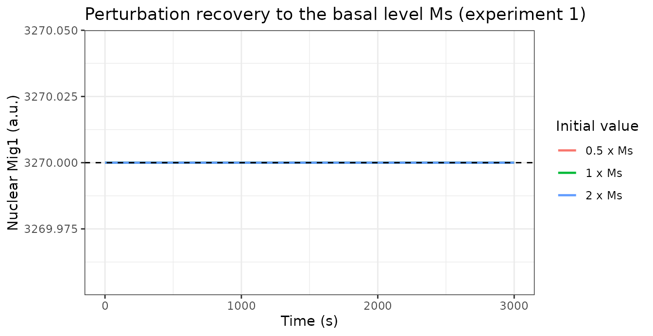
Replicating Figure 4: typical cell and individual cells
Figure 4 of the paper shows, in its first row, the simulated “typical
cell” (all random effects set to zero) for each experiment overlaid on
the observed single-cell data, and in rows two to five the
empirical-Bayes fits of representative individual cells. The raw
single-cell data are not redistributed with nlmixr2lib, so
the panels below overlay simulated cells drawn from the estimated
population distribution in place of the observed data.
glucose_label <- c(exp1 = "Exp 1: 4% -> 1.5%", exp2 = "Exp 2: 4% -> 1.5%",
                   exp3 = "Exp 3: 4% -> 1%",   exp4 = "Exp 4: 4% -> 0.5%")

# 20 simulated cells per experiment, plus the typical cell.
grid_20min <- rxode2::et(seq(-30, 1200, by = 5))

cells <- bind_rows(lapply(names(ui), function(nm) {
  ev <- rxode2::et(grid_20min) |> rxode2::et(id = 1:20)
  s  <- rxode2::rxSolve(ui[[nm]], ev, returnType = "data.frame")
  data.frame(Experiment = glucose_label[[nm]], id = s$id, time = s$time,
             mig1 = s$mig1, obs = s$sim)
}))

typical <- bind_rows(lapply(names(ui), function(nm) {
  s <- rxode2::rxSolve(rxode2::zeroRe(ui[[nm]]), grid_20min, returnType = "data.frame")
  data.frame(Experiment = glucose_label[[nm]], time = s$time, mig1 = s$mig1)
}))
#> ℹ omega/sigma items treated as zero: 'etalrbase', 'etalkout_mig1', 'etalkout_adapt'
#> ℹ omega/sigma items treated as zero: 'etalrbase', 'etalkout_mig1', 'etalkout_adapt'
#> ℹ omega/sigma items treated as zero: 'etalrbase', 'etalkout_mig1', 'etalkout_adapt'
#> ℹ omega/sigma items treated as zero: 'etalrbase', 'etalkout_mig1', 'etalkout_adapt'

ggplot(cells, aes(time, mig1)) +
  geom_line(aes(group = id), colour = "grey65", linewidth = 0.3) +
  geom_line(data = typical, colour = "black", linewidth = 1.1) +
  geom_vline(xintercept = 0, linetype = "dotted") +
  facet_wrap(~Experiment) +
  labs(x = "Time (s)", y = "Nuclear Mig1 (a.u.)",
       title = "Replicates Figure 4, row 1, of Almquist 2015",
       subtitle = "Black: typical cell (all etas zero). Grey: 20 cells drawn from the estimated population.") +
  theme_bw()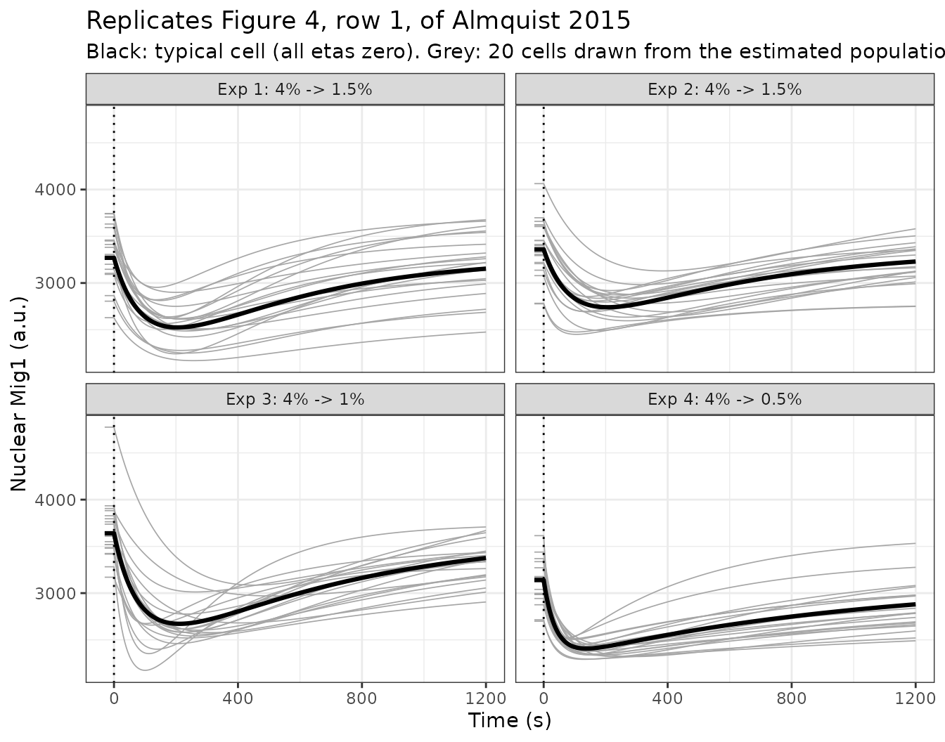
The transient is reproduced in every experiment: a rapid exit from the nucleus, a minimum after roughly two to four minutes, and a slower re-entry towards the pre-shift baseline. The paper reports that the observed intensities recovered to an average of 96% of their pre-shift value by 20 minutes; the typical-cell simulations recover to:
rec20 <- typical |>
  group_by(Experiment) |>
  summarise(`Recovery at 20 min (%)` = round(100 * last(mig1) / first(mig1), 1), .groups = "drop")
knitr::kable(rec20, caption = "Model-predicted recovery of the typical cell at 20 minutes.")| Experiment | Recovery at 20 min (%) |
|---|---|
| Exp 1: 4% -> 1.5% | 96.4 |
| Exp 2: 4% -> 1.5% | 96.1 |
| Exp 3: 4% -> 1% | 92.7 |
| Exp 4: 4% -> 0.5% | 91.7 |
The two 1.5% experiments land essentially on the reported 96%, while the 1% and 0.5% experiments recover less completely by 20 minutes. That ordering is the expected consequence of the paper’s own finding that the duration of the transient lengthens as post-shift glucose falls – the slower experiments simply have not finished re-entering when the recording stops. It is also consistent with the authors’ caveat that “all cells might not fully have completed their re-entry during the course of the experiment”, and with their decision not to model fluorophore bleaching (which would have pushed the observed recovery the other way). Weighted by the cell counts in Table 1, the model’s typical cells average 94% recovery against the reported 96%.
Individual-cell parameter values reported in Figure 6
Figure 6 of the paper compares NLME and standard-two-stage fits for
three specific cells, and prints the NLME (Ms, k2, k4)
triplet used in each panel. These are the only individual-cell parameter
values given in the main text, so they provide a direct check that the
model file accepts and reproduces published per-cell parameters:
fig6 <- data.frame(
  panel = c("6A (information-rich)", "6B (one data point)", "6C (low information)"),
  Ms    = c(3565,    3007,    3360),
  k2    = c(0.00667, 0.00442, 0.00619),
  k4    = c(0.00754, 0.0104,  0.0171)
)

fig6_sim <- bind_rows(lapply(seq_len(nrow(fig6)), function(i) {
  p <- c(lrbase     = log(fig6$Ms[i]),
         lkout_mig1 = log(fig6$k2[i]),
         lkout_adapt = log(fig6$k4[i]))
  s <- rxode2::rxSolve(rxode2::zeroRe(ui$exp1), grid_20min, params = p,
                       returnType = "data.frame")
  data.frame(panel = fig6$panel[i], time = s$time, mig1 = s$mig1,
             baseline = fig6$Ms[i])
}))
#> ℹ omega/sigma items treated as zero: 'etalrbase', 'etalkout_mig1', 'etalkout_adapt'
#> ℹ omega/sigma items treated as zero: 'etalrbase', 'etalkout_mig1', 'etalkout_adapt'
#> ℹ omega/sigma items treated as zero: 'etalrbase', 'etalkout_mig1', 'etalkout_adapt'

ggplot(fig6_sim, aes(time, mig1, colour = panel)) +
  geom_line(linewidth = 0.9) +
  geom_line(data = typical[typical$Experiment == glucose_label[["exp1"]], ],
            aes(time, mig1), colour = "black", linetype = "dashed", inherit.aes = FALSE) +
  geom_vline(xintercept = 0, linetype = "dotted") +
  labs(x = "Time (s)", y = "Nuclear Mig1 (a.u.)", colour = "Almquist 2015 Fig 6 cell",
       title = "Individual cells using the NLME parameter triplets printed in Figure 6",
       subtitle = "Dashed: typical experiment-1 cell, shown for comparison as in the paper") +
  theme_bw()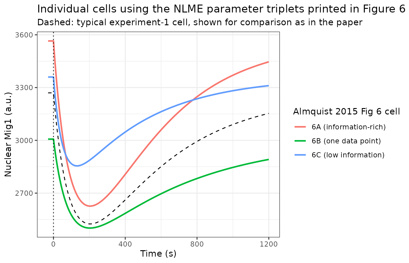
The paper does not state which experiment each Figure 6 cell belongs
to, so the 1.5% post-shift input of experiment 1 is used here; see
Assumptions below. The qualitative ordering the paper describes is
reproduced: the cell in panel 6A, with a k4 below the
typical value, tracks the typical cell closely, while the panel 6C cell
– with k4 roughly twice the typical value – adapts
noticeably faster.
Replicating Figure 7 and Table 5: the predicted distribution of response characteristics
The paper’s headline prediction is obtained by Monte Carlo simulation of the inferred population model. Three characteristics of each simulated cell’s transient are computed (Figure 7A):
- Response time – the time at which nuclear Mig1 reaches its minimum.
- Amplitude – the depth of the minimum, in % below that cell’s own baseline.
- Duration – the total time nuclear Mig1 spends below the half-maximal response level.
Table 5 reports the medians of these distributions, computed by the
authors from 100 000 in-silico cells per experiment.
nlmixr2lib vignettes cap simulated cohorts at 200 per arm,
so the values below carry a Monte Carlo error that the published values
effectively do not; the comparison is calibrated against that error
rather than against an arbitrary fixed tolerance (see the note after the
table).
response_metrics <- function(tt, y) {
  baseline <- y[1]                       # pre-shift level = that cell's own Ms
  i        <- which.min(y)
  minimum  <- y[i]
  half     <- baseline - 0.5 * (baseline - minimum)
  below    <- y < half
  data.frame(
    response_time = tt[i],
    amplitude     = 100 * (baseline - minimum) / baseline,
    duration      = if (any(below)) diff(range(tt[below])) else 0
  )
}

grid_mc <- rxode2::et(seq(-30, 3000, by = 2))

percell <- bind_rows(lapply(names(ui), function(nm) {
  ev <- rxode2::et(grid_mc) |> rxode2::et(id = 1:200)
  s  <- rxode2::rxSolve(ui[[nm]], ev, returnType = "data.frame")
  s |>
    group_by(id) |>
    group_modify(~ response_metrics(.x$time, .x$mig1)) |>
    ungroup() |>
    mutate(Experiment = nm)
}))

# Table 5 groups experiments 1 and 2 into a single 1.5% column; pool them.
percell <- percell |>
  mutate(Condition = case_when(
    Experiment %in% c("exp1", "exp2") ~ "1.5% (exp 1 and 2)",
    Experiment == "exp3"              ~ "1% (exp 3)",
    Experiment == "exp4"              ~ "0.5% (exp 4)"
  ))
percell |>
  pivot_longer(c(response_time, amplitude, duration),
               names_to = "quantity", values_to = "value") |>
  mutate(quantity = recode(quantity,
                           response_time = "Response time (s)",
                           amplitude     = "Amplitude (% below baseline)",
                           duration      = "Duration (s)")) |>
  ggplot(aes(value, colour = Condition)) +
  geom_density(linewidth = 0.8) +
  facet_wrap(~quantity, scales = "free") +
  labs(x = NULL, y = "Density",
       title = "Replicates Figure 7B-D of Almquist 2015") +
  theme_bw() +
  theme(legend.position = "bottom")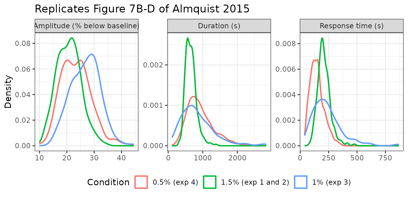
published <- data.frame(
  Condition             = c("1.5% (exp 1 and 2)", "1% (exp 3)", "0.5% (exp 4)"),
  pub_response_time     = c(204, 211, 137),
  pub_amplitude         = c(21,  26,  23),
  pub_duration          = c(639, 758, 844),
  # Monte Carlo SD of the 200-cell (400-cell for the pooled 1.5% column) median,
  # measured across eight independent seeds while preparing this vignette.
  se_response_time      = c(3.1, 16.8, 6.8),
  se_amplitude          = c(0.28, 0.59, 0.56),
  se_duration           = c(7.8, 56.7, 37.0)
)

simulated <- percell |>
  group_by(Condition) |>
  summarise(sim_response_time = median(response_time),
            sim_amplitude     = median(amplitude),
            sim_duration      = median(duration),
            n_cells           = n(),
            .groups = "drop")

cmp <- published |>
  left_join(simulated, by = "Condition") |>
  mutate(across(where(is.numeric), ~ round(.x, 2)))

cmp |>
  transmute(
    Condition,
    `Cells simulated`        = n_cells,
    `Response time, published (s)` = pub_response_time,
    `Response time, simulated (s)` = sim_response_time,
    `Amplitude, published (%)`     = pub_amplitude,
    `Amplitude, simulated (%)`     = sim_amplitude,
    `Duration, published (s)`      = pub_duration,
    `Duration, simulated (s)`      = sim_duration
  ) |>
knitr::kable(caption = "Almquist 2015 Table 5 (Model rows) vs. this implementation.")| Condition | Cells simulated | Response time, published (s) | Response time, simulated (s) | Amplitude, published (%) | Amplitude, simulated (%) | Duration, published (s) | Duration, simulated (s) |
|---|---|---|---|---|---|---|---|
| 1.5% (exp 1 and 2) | 400 | 204 | 202 | 21 | 20.83 | 639 | 636 |
| 1% (exp 3) | 200 | 211 | 213 | 26 | 27.39 | 758 | 741 |
| 0.5% (exp 4) | 200 | 137 | 144 | 23 | 23.18 | 844 | 854 |
The agreement band is set at three Monte Carlo standard errors, where the standard errors were measured empirically by repeating the whole simulation across eight independent seeds. For the amplitude the published value is reported as a whole percent, so half a percentage point of rounding is added to the band.
within_band <- function(sim, pub, se, extra = 0) abs(sim - pub) <= 3 * se + extra

gate <- cmp |>
  transmute(
    Condition,
    response_time = within_band(sim_response_time, pub_response_time, se_response_time),
    amplitude     = within_band(sim_amplitude,     pub_amplitude,     se_amplitude, extra = 0.5),
    duration      = within_band(sim_duration,      pub_duration,      se_duration)
  )
knitr::kable(gate, caption = "Each simulated median within 3 Monte Carlo SE of the published value.")| Condition | response_time | amplitude | duration |
|---|---|---|---|
| 1.5% (exp 1 and 2) | TRUE | TRUE | TRUE |
| 1% (exp 3) | TRUE | TRUE | TRUE |
| 0.5% (exp 4) | TRUE | TRUE | TRUE |
The three qualitative conclusions the paper draws from Figure 7 also hold in the reproduction: the median response time falls markedly at 0.5% glucose, the amplitude is largely independent of the glucose level, and the duration increases steadily as glucose decreases.
trend <- simulated |>
  mutate(Condition = factor(Condition,
                            levels = c("1.5% (exp 1 and 2)", "1% (exp 3)", "0.5% (exp 4)"))) |>
  arrange(Condition)

# Duration increases monotonically as post-shift glucose decreases.
stopifnot(all(diff(trend$sim_duration) > 0))
# Response time at 0.5% is the fastest of the three conditions.
stopifnot(which.min(trend$sim_response_time) == 3L)
# Amplitude varies little across conditions (paper: "largely independent").
stopifnot(diff(range(trend$sim_amplitude)) < 10)
Assumptions and deviations
Only the four per-experiment fits are packaged. The paper also reports two variants: a simultaneous fit of all four data sets (S2 Text, S4 and S5 Tables) and a fit with an added background-fluorescence parameter (S1 Text, S2 and S3 Tables). Neither is packaged. The simultaneous fit is not, because the authors themselves conclude that “the results from the separate analysis should be considered more trustworthy” – the experiment-4 empirical Bayes estimates form a separate cluster, violating the assumption that the random effects are identically distributed across experiments. The background-fluorescence variant is not, because the authors report that its “parameter estimation suffered from issues with practical identifiability and this model variant was therefore not considered further”. The numeric values for both variants live only in the supplementary tables, which were not available when this model was built.
Omegais reconstructed rather than transcribed. The packaged covariance matrices are built from the Table 2 decomposition parameters viaOmega = U %*% t(U), not typed in from the two-significant-figure Table 3 print. The reconstruction is verified against Table 3 above (covariances and correlations both). This gains roughly one significant figure and guarantees positive definiteness.sis treated as a variance. See the Source trace section. The additive residual SD in the model file issqrt(s).Figure 6 cells are simulated under the 1.5% input. The paper prints the NLME
(Ms, k2, k4)triplets for its three Figure 6 cells but does not say which experiment each came from, and the post-shift glucose level changes the trajectory. Experiment 1’s 1.5% input is used; the panel is illustrative of the individual-parameter mechanism, not a quantitative reproduction of Figure 6.Observed single-cell data are not redistributed. The paper’s Figures 1 and 4 overlay the raw fluorescence time series, which are not included in
nlmixr2lib. The Figure 4 replication above substitutes cells simulated from the estimated population distribution.Empirical Bayes estimates are not packaged. Per-cell EBEs appear only in supplementary figures S1 to S4 (as plots, not tables) and are therefore not recoverable as numbers from the main text.
Monte Carlo cohort size. The paper used 100 000 in-silico cells per experiment; this vignette uses 200 per experiment to respect the package’s cohort cap. The Table 5 comparison is therefore calibrated to the measured Monte Carlo standard error of the 200-cell median rather than to a fixed percentage tolerance.
Convention check.
checkModelConventions()reports one warning per model file: the single-output observation variablemig1is not a registered canonical output name. It is deliberately retained. The observed quantity is nuclear Mig1-GFP light intensity, which is neither a plasma drug concentration (Cc) nor any currently registered PD-output compartment;mig1andadaptare declared through thepaper_specific_compartmentsmechanism, following the precedent of the Bizzotto 2016 glucose-insulin phase states and the Denti 2010insulin_actionstate. Registeringmig1as a canonical PD-output compartment (as was done forlogfluorin the Frohlich 2018 single-cell model) would clear the warning and is the natural follow-up if the maintainers want it silenced.No errata. No correction, corrigendum or expression of concern was found for this article on the PLOS ONE landing page or in PubMed.
Session info
sessionInfo()
#> R version 4.6.1 (2026-06-24)
#> Platform: x86_64-pc-linux-gnu
#> Running under: Ubuntu 24.04.5 LTS
#>
#> Matrix products: default
#> BLAS:   /usr/lib/x86_64-linux-gnu/openblas-pthread/libblas.so.3
#> LAPACK: /usr/lib/x86_64-linux-gnu/openblas-pthread/libopenblasp-r0.3.26.so;  LAPACK version 3.12.0
#>
#> locale:
#>  [1] LC_CTYPE=C.UTF-8       LC_NUMERIC=C           LC_TIME=C.UTF-8
#>  [4] LC_COLLATE=C.UTF-8     LC_MONETARY=C.UTF-8    LC_MESSAGES=C.UTF-8
#>  [7] LC_PAPER=C.UTF-8       LC_NAME=C              LC_ADDRESS=C
#> [10] LC_TELEPHONE=C         LC_MEASUREMENT=C.UTF-8 LC_IDENTIFICATION=C
#>
#> time zone: UTC
#> tzcode source: system (glibc)
#>
#> attached base packages:
#> [1] stats     graphics  grDevices utils     datasets  methods   base
#>
#> other attached packages:
#> [1] ggplot2_4.0.3         tidyr_1.3.2           dplyr_1.2.1
#> [4] rxode2_5.1.8          nlmixr2lib_0.3.2.9000
#>
#> loaded via a namespace (and not attached):
#>  [1] generics_0.1.4      sass_0.4.10         xml2_1.6.0
#>  [4] digest_0.6.39       magrittr_2.0.5      RColorBrewer_1.1-3
#>  [7] evaluate_1.0.5      grid_4.6.1          fastmap_1.2.0
#> [10] lotri_1.0.5         jsonlite_2.0.0      whisker_0.4.1
#> [13] rxode2ll_2.0.18     backports_1.5.1     purrr_1.2.2
#> [16] scales_1.4.0        textshaping_1.0.5   jquerylib_0.1.4
#> [19] cli_3.6.6           crayon_1.5.3        symengine_0.2.14
#> [22] rlang_1.3.0         withr_3.0.3         cachem_1.1.0
#> [25] yaml_2.3.12         otel_0.2.0          tools_4.6.1
#> [28] parallel_4.6.1      memoise_2.0.1       checkmate_2.3.4
#> [31] rxode2lincmt_0.1.0  vctrs_0.7.3         R6_2.6.1
#> [34] lifecycle_1.0.5     fs_2.1.0            ragg_1.5.2
#> [37] PreciseSums_0.7     fontawesome_0.5.3   pkgconfig_2.0.3
#> [40] desc_1.4.3          rex_1.2.2           pkgdown_2.2.1
#> [43] pillar_1.11.1       bslib_0.12.0        gtable_0.3.6
#> [46] glue_1.8.1          data.table_1.18.6.1 Rcpp_1.1.2
#> [49] systemfonts_1.3.2   tidyselect_1.2.1    xfun_0.61
#> [52] tibble_3.3.1        sys_3.4.3           knitr_1.52
#> [55] farver_2.1.2        dparser_1.3.1-14    htmltools_0.5.9
#> [58] labeling_0.4.3      rmarkdown_2.32      compiler_4.6.1
#> [61] S7_0.2.2            downlit_0.4.5       askpass_1.2.1
#> [64] openssl_2.4.2