Dexketoprofen CAT-PBPK (Zhang 2022)
Source:vignettes/articles/Zhang_2022_dexketoprofen_pbpk.Rmd
Zhang_2022_dexketoprofen_pbpk.RmdModel and source
- Citation: Zhang X, Ye X, Hu K, Li W, Li W, Xiao Q, Chen L, Yang J (2022). A Physiologically Based Pharmacokinetic Model for Studying the Biowaiver Risk of Biopharmaceutics Classification System Class I Drugs With Rapid Elimination: Dexketoprofen Trometamol Case Study. Front Pharmacol 13:808456. doi:10.3389/fphar.2022.808456. MMC gastric-emptying inputs from Oberle RL et al. (1990) The influence of the interdigestive migrating myoelectric complex on the gastric emptying of liquids. Gastroenterology 99(5):1275-1282. doi:10.1016/0016-5085(90)91150-5.
- Description: PBPK (compartmental absorption and transit (CAT) model, Berkeley Madonna 8.3.18). Oral dexketoprofen (as dexketoprofen trometamol immediate-release tablet) in fasted healthy adults. The gastrointestinal tract is one stomach segment and seven equal small-intestinal transit segments, each split into undissolved and dissolved drug (Eqs 1-4, Figure 2). Undissolved drug dissolves first-order with a pH-specific rate constant (pH 1.2 in the stomach, pH 4.5 in segment 1, pH 6.8 in segments 2-7), empties from the stomach at the solid (undissolved) or liquid (dissolved) gastric emptying rate, and transits the intestine at a common rate; only dissolved drug in the intestinal segments is absorbed, at Ka = 2 * Peff / R (Eq 7). Absorbed drug enters a two-compartment disposition model fitted to intravenous data. Deterministic: the paper’s between-subject variability is a Monte Carlo draw of the liquid gastric emptying rate from a migrating myoelectric complex (MMC) model, implemented in the validation vignette as a per-subject value of lkst_liquid.
- Article: https://doi.org/10.3389/fphar.2022.808456 (open access, with Supplementary Data Sheet 1)
- Gastric-emptying inputs: Oberle et al. (1990), https://doi.org/10.1016/0016-5085(90)91150-5, Table 2 and the Results text on the migrating myoelectric complex (MMC) phase durations.
Zhang et al. (2022) built a compartmental absorption and transit (CAT) model for dexketoprofen trometamol, a BCS class I drug with rapid elimination, to ask whether the BCS-based biowaiver is safe for it. The stomach and seven small-intestinal segments each hold an undissolved and a dissolved pool; dissolution is first order with a rate constant that depends on the pH of the segment; only dissolved drug in the intestine is absorbed. Absorbed drug enters a two-compartment disposition model that the authors fitted to intravenous data. The authors then (i) ran a one-at-a-time sensitivity analysis, (ii) added a “gastric emptying variation model” that draws the liquid gastric emptying rate from the phase of the migrating myoelectric complex at the time of dosing, and (iii) used it to simulate virtual two-period crossover bioequivalence (BE) trials of faster- and slower-dissolving tablets.
The packaged model is the deterministic ODE system. The gastric
emptying variation model is a per-subject draw of one model parameter,
lkst_liquid, and is implemented below as an R function
whose output is passed to rxSolve().
mod <- readModelDb("Zhang_2022_dexketoprofen_pbpk")
ui <- rxode2::rxode2(mod)
theta <- ui$theta
Population
The model is not a population fit. Its pieces come from separate literature sources:
- Disposition (Vc, K10, K12, K21): fitted in Phoenix WinNonlin 7.0 to the mean profile after a 37 mg dexketoprofen trometamol (25 mg dexketoprofen) intravenous bolus in healthy subjects (Valles 2006, n = 12; Supplementary Figure S4).
- Oral verification: mean profiles after 37 mg dexketoprofen trometamol tablets (Barbanoj 1998, n = 18, Figure 3) and 18.5 mg tablets (Mauleon 1996), fasted healthy volunteers (Supplementary Table S3).
- Dissolution: Garcia-Arieta 2015 USP apparatus 2 profiles of the reference tablet at pH 1.2, 4.5 and 6.8 (Supplementary Figure S1).
- Gastric emptying variability: Oberle 1990, seven healthy volunteers with duodenal aspiration and antral manometry after 50 mL and 200 mL phenol-red doses in the fasted state.
Source trace
| Element | Value | Source |
|---|---|---|
| Stomach equations | Eqs 1-2 | Methods, Figure 2 |
| Intestinal equations, 7 segments | Eqs 3-4 | Methods, Figure 2 |
| Ka = 2 * Peff / R | Eq 7 | Methods |
| Liquid gastric emptying from T1/2 | Eqs 5-6 | Methods |
lkdiss_stomach |
8.16 1/h | Table 1, Kdis (pH 1.2) |
lkdiss_duodenum |
6.59 1/h | Table 1, Kdis (pH 4.5) |
lkdiss_intestine |
8.29 1/h | Table 1, Kdis (pH 6.8) |
| pH-to-segment mapping | pH 1.2 stomach, 4.5 segment 1, 6.8 segments 2-7 | Methods, text after Table 2 |
lkst_solid |
1.65 1/h | Table 1, Ktgs |
lkst_liquid |
5.67 1/h | Table 1, Ktgl (footnote a) |
lktr |
2.10 1/h | Table 1, Kt |
lpeff |
3.37 cm/h | Table 1, predicted Peff,man |
lr_intestine |
1.14 cm | Not printed; back-solved (see below) |
lvc |
3.55 L | Table 1, Vc |
lkel |
1.68 1/h | Table 1, K10 |
lk12 |
1.14 1/h | Table 1, K12 |
lk21 |
1.24 1/h | Table 1, K21 |
| MMC phase log10-durations | 1.6 +/- 0.26, 1.9 +/- 0.34, 0.81 +/- 0.24 (log10 min) | Methods “Virtual BE Simulation”; Oberle 1990 Results |
| Gastric emptying rate by phase, 200 mL | 0.104 +/- 0.0014, 0.110 +/- 0.041, 0.236 +/- 0.069 1/min | Oberle 1990 Table 2 (phases I, II, late II/III); Supplementary Figure S3 |
| Draw within +/- 2 SD of each phase mean | uniform | Methods “Virtual BE Simulation” |
| Validation targets | Cmax, AUCtlast | Supplementary Table S3 |
| Sensitivity targets | Ktgl 1.89 -> Cmax 2.10; Ktgl 17.01 -> Cmax 3.33 mg/L | Results “Sensitivity Analysis” |
The intestinal radius R
Equation 7 computes Ka from Peff and the intestinal radius R, but no value of R is printed anywhere in the article or its supplement, and Ka itself is not tabulated. The maintainers back-solved R from the paper’s own model outputs with every other Table 1 value fixed:
- Supplementary Table S3 simulated Cmax 2.90 mg/L after 25 mg gives Ka = 5.91 1/h, i.e. R = 6.74 / 5.91 = 1.14 cm.
- Figure 7B (about 70% of the dose absorbed in intestinal segment 1) independently gives R between 1.13 and 1.19 cm.
- The commonly quoted CAT radius of 1.75 cm is ruled out: it gives Cmax 2.62 mg/L and only 62% absorbed in segment 1.
The checks below show that R = 1.14 cm also reproduces the 12.5 mg Cmax, both AUCtlast values and the Ktgl sensitivity values, none of which were used to back-solve it.
Deterministic replication
Figure 3 and Supplementary Table S3
t_grid <- sort(unique(c(seq(0, 2, by = 0.01), seq(2, 8, by = 0.05))))
ev_det <- bind_rows(
  data.frame(id = 1L, time = 0, amt = 25, evid = 1L, cmt = "stomach_undissolved", treatment = "25 mg"),
  data.frame(id = 1L, time = t_grid, amt = 0, evid = 0L, cmt = "central", treatment = "25 mg"),
  data.frame(id = 2L, time = 0, amt = 12.5, evid = 1L, cmt = "stomach_undissolved", treatment = "12.5 mg"),
  data.frame(id = 2L, time = t_grid, amt = 0, evid = 0L, cmt = "central", treatment = "12.5 mg")
)
# No random effects are present, so rxSolve's multi-subject note about a
# missing omega is expected and suppressed here and below.
sim_det <- suppressWarnings(as.data.frame(rxSolve(mod, ev_det, keep = "treatment")))

# Barbanoj 1998 mean observed profile (n = 18), digitised by the maintainers
# from Figure 3.
obs_fig3 <- data.frame(
  time = c(0.25, 0.5, 0.75, 1, 1.25, 1.5, 1.75, 2, 2.5, 3, 4, 6, 8),
  Cc = c(1.42, 2.89, 2.30, 1.76, 1.34, 1.08, 0.86, 0.70, 0.48, 0.31, 0.18, 0.10, 0.05)
)
ggplot(filter(sim_det, treatment == "25 mg"), aes(time, Cc)) +
  geom_line() +
  geom_point(data = obs_fig3, shape = 16) +
  labs(x = "Time (h)", y = "Dexketoprofen plasma concentration (mg/L)")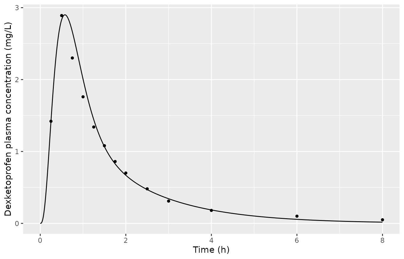
Replicates the black line and the observed means of Figure 3 of Zhang 2022 (25 mg dexketoprofen, fasted).
conc_det <- sim_det |>
  filter(!is.na(Cc)) |>
  select(id, time, Cc, treatment)
dose_det <- ev_det |>
  filter(evid == 1) |>
  select(id, time, amt, treatment)

intervals_det <- data.frame(start = 0, end = 8, cmax = TRUE, tmax = TRUE, auclast = TRUE)
nca_det <- pk.nca(PKNCAdata(
  PKNCAconc(conc_det, Cc ~ time | treatment + id),
  PKNCAdose(dose_det, amt ~ time | treatment + id),
  intervals = intervals_det
))

# Supplementary Table S3: the paper's simulated values (the model being
# reproduced) and the observed means.
ref_s3_sim <- data.frame(treatment = c("25 mg", "12.5 mg"), cmax = c(2.90, 1.45), auclast = c(4.17, 2.09))
ref_s3_obs <- data.frame(treatment = c("25 mg", "12.5 mg"), cmax = c(3.10, 1.38), auclast = c(4.03, 1.66))

cmp_sim <- ncaComparisonTable(
  nca_det, ref_s3_sim,
  by = "treatment", params = c("cmax", "auclast"),
  units = c(cmax = "mg/L", auclast = "mg*h/L"), tolerance_pct = 20
)
knitr::kable(cmp_sim, caption = "Packaged model against the paper's own simulated values, Supplementary Table S3 (AUC over 0-8 h).")| NCA parameter | treatment | Reference | Simulated | % diff |
|---|---|---|---|---|
| Cmax (mg/L) | 25 mg | 2.9 | 2.9 | +0.0% |
| Cmax (mg/L) | 12.5 mg | 1.45 | 1.45 | +0.0% |
| AUClast (mg*h/L) | 25 mg | 4.17 | 4.16 | -0.2% |
| AUClast (mg*h/L) | 12.5 mg | 2.09 | 2.08 | -0.4% |
cmp_obs <- ncaComparisonTable(
  nca_det, ref_s3_obs,
  by = "treatment", params = c("cmax", "auclast"),
  units = c(cmax = "mg/L", auclast = "mg*h/L"), tolerance_pct = 20
)
knitr::kable(cmp_obs, caption = "Packaged model against the observed means, Supplementary Table S3.")| NCA parameter | treatment | Reference | Simulated | % diff |
|---|---|---|---|---|
| Cmax (mg/L) | 25 mg | 3.1 | 2.9 | -6.4% |
| Cmax (mg/L) | 12.5 mg | 1.38 | 1.45 | +5.1% |
| AUClast (mg*h/L) | 25 mg | 4.03 | 4.16 | +3.3% |
| AUClast (mg*h/L) | 12.5 mg | 1.66 | 2.08 | +25.4%* |
res_det <- as.data.frame(nca_det$result)
get_nca <- function(trt, code) res_det$PPORRES[res_det$treatment == trt & res_det$PPTESTCD == code]
# Deterministic solves: the only difference from the paper is rounding of the
# printed values and the back-solved R, so the bounds are tight.
stopifnot(
  abs(get_nca("25 mg", "cmax") / 2.90 - 1) < 0.01,
  abs(get_nca("12.5 mg", "cmax") / 1.45 - 1) < 0.01,
  abs(get_nca("25 mg", "auclast") / 4.17 - 1) < 0.02,
  abs(get_nca("12.5 mg", "auclast") / 2.09 - 1) < 0.02
)
The packaged model reproduces the paper’s simulated Cmax and AUCtlast for both doses. Against the observed means, the 12.5 mg AUCtlast is 25% above the observation; the paper reports a 25.7% prediction error for its own model.
Sensitivity analysis (Figure 4A and 4B)
Each parameter is scaled from 33.3% to 300% of its baseline, as in Table 2, and Cmax and AUCtlast (0-8 h) are normalised to the baseline values.
sens_params <- c(
  "Dissolution rate at pH 1.2" = "lkdiss_stomach",
  "Dissolution rate at pH 4.5" = "lkdiss_duodenum",
  "Dissolution rate at pH 6.8" = "lkdiss_intestine",
  "Peff" = "lpeff",
  "Liquid gastric emptying rate" = "lkst_liquid",
  "Solid gastric emptying rate" = "lkst_solid"
)
scales <- c(1 / 3, 0.5, 0.75, 1, 1.5, 2, 3)
sens_grid <- expand.grid(scale = scales, label = names(sens_params), stringsAsFactors = FALSE)
sens_grid$id <- seq_len(nrow(sens_grid))
sens_grid$param <- sens_params[sens_grid$label]

# One subject per (parameter, scale); every other parameter at its baseline.
sens_par <- data.frame(id = sens_grid$id)
for (p in unique(sens_params)) {
  sens_par[[p]] <- theta[[p]] + ifelse(sens_grid$param == p, log(sens_grid$scale), 0)
}
ev_sens <- et(amt = 25, cmt = "stomach_undissolved") |>
  et(t_grid) |>
  et(id = sens_grid$id)
sim_sens <- suppressWarnings(as.data.frame(rxSolve(mod, ev_sens, params = sens_par)))

sens_metrics <- sim_sens |>
  group_by(id) |>
  summarise(
    cmax = max(Cc),
    auclast = sum(diff(time) * (head(Cc, -1) + tail(Cc, -1)) / 2),
    .groups = "drop"
  ) |>
  left_join(sens_grid, by = "id")
base_metrics <- sens_metrics |> filter(scale == 1) |> slice(1)
sens_metrics <- sens_metrics |>
  mutate(cmax_ratio = cmax / base_metrics$cmax, auc_ratio = auclast / base_metrics$auclast)
sens_metrics |>
  select(label, scale, Cmax = cmax_ratio, AUCtlast = auc_ratio) |>
  pivot_longer(c(Cmax, AUCtlast), names_to = "metric", values_to = "ratio") |>
  ggplot(aes(scale, ratio, colour = label)) +
  geom_line() +
  geom_hline(yintercept = c(0.8, 1.25), linetype = "dashed") +
  scale_x_log10(breaks = c(1 / 3, 0.5, 1, 2, 3), labels = c("0.33", "0.5", "1", "2", "3")) +
  facet_wrap(~metric) +
  labs(x = "Baseline-normalised parameter", y = "Normalised PK metric", colour = NULL) +
  theme(legend.position = "bottom")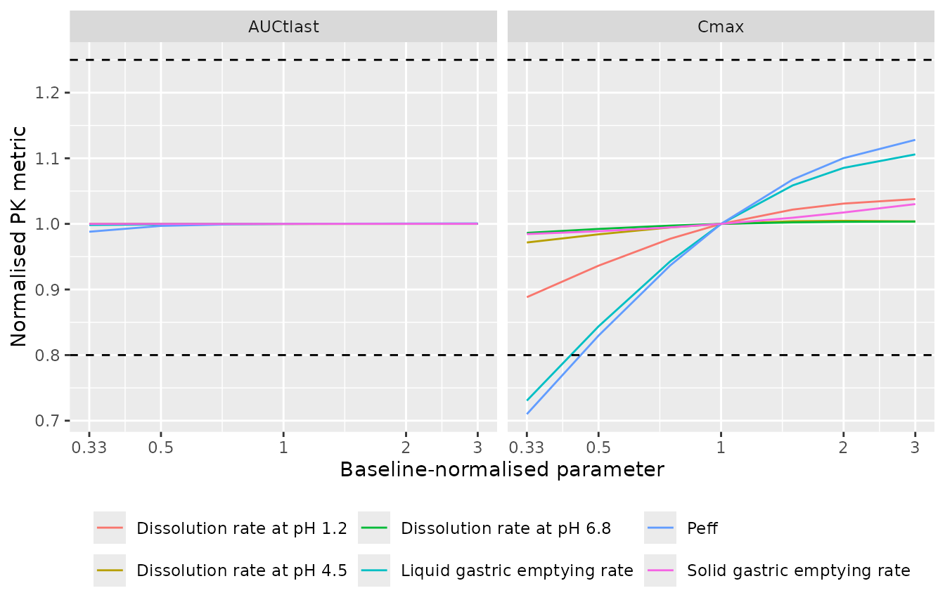
Replicates Figure 4A and 4B of Zhang 2022: normalised Cmax and AUCtlast against the normalised parameter value, with the 80-125% limits dashed.
The Results section prints two absolute values from this analysis: Cmax 2.10 and 3.33 mg/L when Ktgl is set to 1.89 and 17.01 1/h.
cmax_ktgl <- sens_metrics |>
  filter(param == "lkst_liquid", scale %in% c(1 / 3, 3)) |>
  arrange(scale) |>
  pull(cmax)
knitr::kable(
  data.frame(Ktgl = c(1.89, 17.01), Paper = c(2.10, 3.33), Model = round(cmax_ktgl, 2)) |>
    dplyr::rename("Ktgl (1/h)" = Ktgl, "Paper Cmax (mg/L)" = Paper, "Model Cmax (mg/L)" = Model),
  caption = "Cmax at the Table 2 limits of the liquid gastric emptying rate."
)| Ktgl (1/h) | Paper Cmax (mg/L) | Model Cmax (mg/L) |
|---|---|---|
| 1.89 | 2.10 | 2.12 |
| 17.01 | 3.33 | 3.21 |
Both are within 4%. Dissolution at pH 1.2, Peff and Ktgl move Cmax, while dissolution at pH 4.5 and 6.8 and AUCtlast barely respond, which is the pattern of Figure 4A and 4B.
Dissolution and absorption by segment (Figure 7)
Figure 7 splits the dose dissolved and absorbed by segment for the
reference (“medium”) tablet and for the faster and slower tablets used
in the virtual BE trials. The amounts are the time integrals of the
dissolution flux kdiss * undissolved and of the absorption
flux ka * dissolved in each segment.
The fast and slow tablets are defined in the paper as the two first-order profiles with a similarity factor f2 of exactly 50 against the reference at pH 1.2 (Equation 9; Supplementary Figure S5). Their rate constants are not printed. The maintainers solved f2 = 50 against the reference tablet’s observed pH 1.2 profile (Supplementary Figure S1a, six points digitised at 5-30 min).
# Reference tablet at pH 1.2, Supplementary Figure S1a, digitised.
diss_ref <- data.frame(time_min = c(5, 10, 15, 20, 25, 30), pct = c(40.5, 79.2, 91.5, 94.7, 96.8, 98.1))
f2 <- function(k_test) {
  test <- 100 * (1 - exp(-k_test * diss_ref$time_min / 60))
  50 * log10(100 / sqrt(1 + mean((diss_ref$pct - test)^2)))
}
k_fast <- uniroot(function(k) f2(k) - 50, c(8.2, 60))$root
k_slow <- uniroot(function(k) f2(k) - 50, c(1, 8.1))$root
formulations <- c(Fast = k_fast, Medium = exp(theta[["lkdiss_stomach"]]), Slow = k_slow)
round(formulations, 2)
#>   Fast Medium   Slow
#>  11.96   8.16   5.91
t_fine <- seq(0, 24, by = 0.002)
ev7 <- et(amt = 25, cmt = "stomach_undissolved") |>
  et(t_fine) |>
  et(id = 1:3)
par7 <- data.frame(id = 1:3, lkdiss_stomach = log(formulations))
sim7 <- suppressWarnings(as.data.frame(rxSolve(mod, ev7, params = par7)))

ka_val <- 2 * exp(theta[["lpeff"]]) / exp(theta[["lr_intestine"]])
kd_duo <- exp(theta[["lkdiss_duodenum"]])
kd_int <- exp(theta[["lkdiss_intestine"]])
trap <- function(x, y) sum(diff(x) * (head(y, -1) + tail(y, -1)) / 2)
seg_fractions <- function(d) {
  kd_sto <- formulations[[unique(d$id)]]
  dissolved <- c(
    Stomach = trap(d$time, kd_sto * d$stomach_undissolved),
    sapply(1:7, function(n) trap(d$time, ifelse(n == 1, kd_duo, kd_int) * d[[paste0("intestine", n, "_undissolved")]]))
  )
  absorbed <- sapply(1:7, function(n) trap(d$time, ka_val * d[[paste0("intestine", n, "_dissolved")]]))
  data.frame(
    segment = c("Stomach", paste("Intestine", 1:7), paste("Intestine", 1:7)),
    process = rep(c("Dissolved", "Absorbed"), c(8, 7)),
    pct = 100 * c(dissolved, absorbed) / 25
  )
}
fig7 <- sim7 |>
  group_by(id) |>
  group_modify(~ seg_fractions(cbind(.x, id = .y$id))) |>
  ungroup() |>
  mutate(formulation = names(formulations)[id])
fig7 |>
  mutate(segment = factor(segment, levels = c("Stomach", paste("Intestine", 1:7)))) |>
  ggplot(aes(segment, pct, fill = formulation)) +
  geom_col(position = "dodge") +
  facet_wrap(~process, scales = "free_x") +
  labs(x = NULL, y = "Percent of dose", fill = NULL) +
  theme(axis.text.x = element_text(angle = 45, hjust = 1))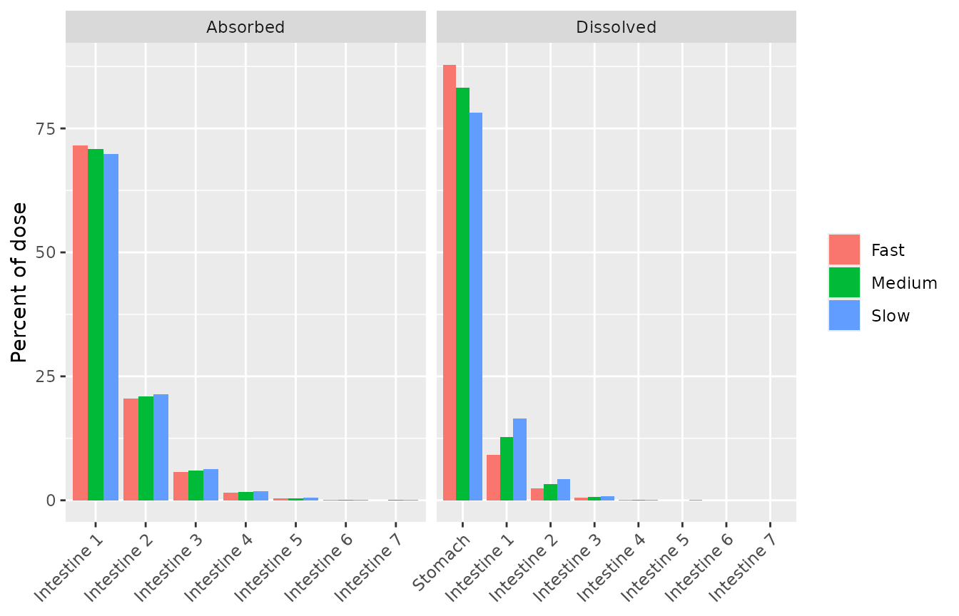
Replicates Figure 7 of Zhang 2022: percent of the 25 mg dose dissolved (A) and absorbed (B) in each segment.
fig7_tab <- fig7 |>
  select(-id) |>
  filter(segment %in% c("Stomach", "Intestine 1", "Intestine 2")) |>
  mutate(pct = round(pct, 1)) |>
  pivot_wider(names_from = formulation, values_from = pct) |>
  dplyr::rename("Process" = process, "Segment" = segment)
knitr::kable(fig7_tab, caption = "Percent of dose by segment. Figure 7, read by the maintainers: dissolved in the stomach about 87 / 83 / 78% and in segment 1 about 10 / 13 / 17% (fast / medium / slow); absorbed in segment 1 about 71 / 70 / 69%.")| Segment | Process | Fast | Medium | Slow |
|---|---|---|---|---|
| Stomach | Dissolved | 87.9 | 83.2 | 78.2 |
| Intestine 1 | Dissolved | 9.2 | 12.8 | 16.5 |
| Intestine 2 | Dissolved | 2.3 | 3.2 | 4.2 |
| Intestine 1 | Absorbed | 71.6 | 70.8 | 69.9 |
| Intestine 2 | Absorbed | 20.5 | 20.9 | 21.4 |
med <- filter(fig7, formulation == "Medium")
stopifnot(
  abs(med$pct[med$process == "Dissolved" & med$segment == "Stomach"] - 83.2) < 1,
  abs(med$pct[med$process == "Absorbed" & med$segment == "Intestine 1"] - 70) < 3,
  abs(sum(med$pct[med$process == "Absorbed"]) - 100) < 1
)
The reference tablet dissolves 83% in the stomach and absorbs about 70% of the dose in segment 1, as the Discussion states (“more than 75% of the drugs were dissolved in the stomach, and more than 70% of the drugs were absorbed in the first intestinal segment”). The fast and slow profiles from the f2 solution give stomach fractions that agree with Figure 7A to within about 1 percentage point.
Gastric emptying variation model
Construction
The paper’s gastric emptying variation model, rebuilt from its Methods text and the Oberle 1990 data it cites:
- Each subject has lognormal durations for MMC phases I, II and III, with log10-scale mean and SD 1.6 +/- 0.26, 1.9 +/- 0.34 and 0.81 +/- 0.24 (minutes). The cycle is their sum. A subject keeps the same durations in every period of a crossover.
- At each dose the dosing time falls uniformly within that subject’s cycle, which fixes the MMC phase at dosing.
- The liquid gastric emptying rate is drawn uniformly within +/- 2 SD of the Oberle 1990 Table 2 mean for that phase, for the 200 mL volume: phase I 0.104 +/- 0.0014, phase II 0.110 +/- 0.041, late phase II/III 0.236 +/- 0.069 1/min. Supplementary Figure S3 plots exactly these three means and SDs in 1/h as the “observed” bars.
mmc_durations <- function(n) {
  data.frame(
    d1 = 10^rnorm(n, 1.6, 0.26),
    d2 = 10^rnorm(n, 1.9, 0.34),
    d3 = 10^rnorm(n, 0.81, 0.24)
  )
}
mmc_phase <- function(dur) {
  u <- runif(nrow(dur)) * (dur$d1 + dur$d2 + dur$d3)
  ifelse(u < dur$d1, 1L, ifelse(u < dur$d1 + dur$d2, 2L, 3L))
}
# Oberle 1990 Table 2 (200 mL), 1/min converted to 1/h.
ge_mean <- c(0.104, 0.110, 0.236) * 60
ge_sd <- c(0.0014, 0.041, 0.069) * 60
draw_ktgl <- function(phase) {
  runif(length(phase), ge_mean[phase] - 2 * ge_sd[phase], ge_mean[phase] + 2 * ge_sd[phase])
}
Checks against Supplementary Tables S1 and S2 and Figure S3
All randomness here and in the cohorts below comes from base R’s generator, and the rxode2 solves are deterministic given the drawn rates, so the results do not depend on the solver’s thread count.
set.seed(808456)
n_mc <- 100000
dur_mc <- mmc_durations(n_mc)
phase_mc <- mmc_phase(dur_mc)
ktgl_mc <- draw_ktgl(phase_mc)

tab_s1 <- data.frame(
  Phase = c("I", "II", "III", "Cycle"),
  Paper = c("47.8 +/- 31.5", "107.9 +/- 98.4", "7.5 +/- 4.4", "163.2 +/- 103.7"),
  Model = sprintf(
    "%.1f +/- %.1f",
    c(mean(dur_mc$d1), mean(dur_mc$d2), mean(dur_mc$d3), mean(rowSums(dur_mc))),
    c(sd(dur_mc$d1), sd(dur_mc$d2), sd(dur_mc$d3), sd(rowSums(dur_mc)))
  )
) |>
  dplyr::rename("Paper, simulated (min)" = Paper, "Model (min)" = Model)
knitr::kable(tab_s1, caption = "MMC phase durations: Supplementary Table S1 simulated column against this implementation.")| Phase | Paper, simulated (min) | Model (min) |
|---|---|---|
| I | 47.8 +/- 31.5 | 47.7 +/- 31.3 |
| II | 107.9 +/- 98.4 | 107.9 +/- 99.5 |
| III | 7.5 +/- 4.4 | 7.5 +/- 4.5 |
| Cycle | 163.2 +/- 103.7 | 163.2 +/- 104.5 |
tab_s3 <- data.frame(
  Phase = c("I", "II", "III (late II/III)"),
  Mean = tapply(ktgl_mc, phase_mc, mean),
  SD = tapply(ktgl_mc, phase_mc, sd)
) |>
  mutate(Mean = round(Mean, 2), SD = round(SD, 2)) |>
  dplyr::rename("Mean Ktgl (1/h)" = Mean, "SD Ktgl (1/h)" = SD)
knitr::kable(tab_s3, row.names = FALSE, caption = "Liquid gastric emptying rate by phase; compare the 'simulated' bars of Supplementary Figure S3 (about 6.2, 6.6 +/- 2.8, 14.1 +/- 4.8 1/h).")| Phase | Mean Ktgl (1/h) | SD Ktgl (1/h) |
|---|---|---|
| I | 6.24 | 0.10 |
| II | 6.60 | 2.85 |
| III (late II/III) | 14.15 | 4.79 |
mean_thalf <- mean(log(2) / ktgl_mc)
c(mean_thalf_h = mean_thalf, ktgl_from_mean_thalf = log(2) / mean_thalf)
#>         mean_thalf_h ktgl_from_mean_thalf
#>            0.1228136            5.6438964

stopifnot(
  # Supplementary Table S2: simulated mean liquid gastric emptying half-life 0.122 h
  abs(mean_thalf / 0.122 - 1) < 0.03,
  # Table 1 Ktgl 5.67 = ln(2) / mean half-life (Eqs 5-6, footnote a)
  abs(log(2) / mean_thalf / 5.67 - 1) < 0.03,
  abs(mean(rowSums(dur_mc)) / 163.2 - 1) < 0.03
)
The phase durations match Supplementary Table S1 and the per-phase
rates match Supplementary Figure S3. The mean half-life of 0.123 h and
the derived 5.64 1/h reproduce Supplementary Table S2 (0.122 h) and the
Table 1 value of Ktgl (5.67 1/h). That ties the deterministic model’s
lkst_liquid to the mean of the variation model.
Figure 3 shaded band
n_band <- 200
ktgl_band <- draw_ktgl(mmc_phase(mmc_durations(n_band)))
ev_band <- et(amt = 25, cmt = "stomach_undissolved") |>
  et(seq(0, 8, by = 0.025)) |>
  et(id = seq_len(n_band))
sim_band <- suppressWarnings(as.data.frame(rxSolve(
  mod, ev_band,
  params = data.frame(id = seq_len(n_band), lkst_liquid = log(ktgl_band))
)))
band <- sim_band |>
  group_by(time) |>
  summarise(q05 = quantile(Cc, 0.05), q95 = quantile(Cc, 0.95), .groups = "drop")
ggplot() +
  geom_ribbon(data = band, aes(time, ymin = q05, ymax = q95), fill = "grey70") +
  geom_line(data = filter(sim_det, treatment == "25 mg"), aes(time, Cc)) +
  geom_point(data = obs_fig3, aes(time, Cc)) +
  labs(x = "Time (h)", y = "Dexketoprofen plasma concentration (mg/L)")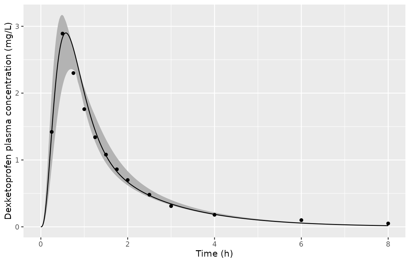
Replicates Figure 3 of Zhang 2022: 5th-95th percentile band of 200 subjects with the gastric emptying variation model (grey), deterministic model (line), Barbanoj 1998 observed means (points).
cmax_band <- sim_band |>
  group_by(id) |>
  summarise(cmax = max(Cc), .groups = "drop")
knitr::kable(
  data.frame(
    Quantity = c("Upper edge of band at its peak", "Lower edge of band at its peak"),
    Paper = c(3.22, 2.04),
    Model = round(c(max(band$q95), max(band$q05)), 2)
  ) |>
    dplyr::rename("Figure 3, read by the maintainers (mg/L)" = Paper, "Model (mg/L)" = Model),
  caption = "Peak of the band edges."
)| Quantity | Figure 3, read by the maintainers (mg/L) | Model (mg/L) |
|---|---|---|
| Upper edge of band at its peak | 3.22 | 3.17 |
| Lower edge of band at its peak | 2.04 | 2.36 |
# The band is a pointwise percentile of a random cohort, so the check is on
# the median Cmax rather than on the band edges.
stopifnot(abs(median(cmax_band$cmax) / 2.90 - 1) < 0.05)
The upper edge of the band matches Figure 3. The lower edge sits about 0.3 mg/L higher than in the figure, so the published band is somewhat wider on the low side than this implementation gives. A per-subject gastric lag time (Oberle 1990 also reports lag times by phase) was tested by the maintainers and makes the lower edge collapse to zero before 0.75 h, which Figure 3 does not show, so lag times are not part of the reconstruction.
Virtual bioequivalence trials (Table 3)
The paper ran 1,000 two-sequence, two-period crossover trials of 24 and 48 subjects for each test tablet (fast, medium, slow) against the reference (medium), and classified each trial by Cmax: BE when the 90% CI of the geometric mean ratio (GMR) lies within 80-125%; “fail to demonstrate BE” when the GMR lies within the limits but the CI does not; “fail to demonstrate BIE” when the GMR lies outside but the CI overlaps the limits; and “demonstrate BIE” when the CI lies entirely outside.
With no residual or other between-occasion variability in the model, Cmax for a given tablet depends only on the drawn Ktgl. The trials below therefore solve the model once on a grid of Ktgl values per tablet and interpolate Cmax for each virtual subject-period, which keeps 1,000 trials cheap.
ktgl_grid <- exp(seq(log(1.5), log(25), length.out = 60))
grid_par <- expand.grid(ktgl = ktgl_grid, formulation = names(formulations), stringsAsFactors = FALSE)
grid_par$id <- seq_len(nrow(grid_par))
ev_grid <- et(amt = 25, cmt = "stomach_undissolved") |>
  et(seq(0, 4, by = 0.005)) |>
  et(id = grid_par$id)
sim_grid <- suppressWarnings(as.data.frame(rxSolve(
  mod, ev_grid,
  params = data.frame(
    id = grid_par$id,
    lkst_liquid = log(grid_par$ktgl),
    lkdiss_stomach = log(formulations[grid_par$formulation])
  )
)))
grid_par <- grid_par |>
  left_join(sim_grid |> group_by(id) |> summarise(cmax = max(Cc), .groups = "drop"), by = "id")
cmax_fun <- lapply(split(grid_par, grid_par$formulation), function(d) splinefun(log(d$ktgl), log(d$cmax)))
be_trial <- function(n_sub, test) {
  dur <- mmc_durations(n_sub)
  seq_tr <- rep(c(TRUE, FALSE), length.out = n_sub)
  k1 <- draw_ktgl(mmc_phase(dur))
  k2 <- draw_ktgl(mmc_phase(dur))
  f_test <- cmax_fun[[test]]
  f_ref <- cmax_fun[["Medium"]]
  lp1 <- ifelse(seq_tr, f_test(log(k1)), f_ref(log(k1)))
  lp2 <- ifelse(seq_tr, f_ref(log(k2)), f_test(log(k2)))
  # Standard 2x2 crossover analysis on log Cmax via within-subject period
  # differences; the treatment effect is test minus reference.
  d <- (lp2 - lp1) / 2
  est <- mean(d[!seq_tr]) - mean(d[seq_tr])
  s2 <- (sum((d[seq_tr] - mean(d[seq_tr]))^2) + sum((d[!seq_tr] - mean(d[!seq_tr]))^2)) / (n_sub - 2)
  se <- sqrt(s2 * (1 / sum(seq_tr) + 1 / sum(!seq_tr)))
  ci <- est + c(-1, 1) * qt(0.95, n_sub - 2) * se
  gmr <- exp(est)
  ci <- exp(ci)
  if (ci[1] >= 0.8 && ci[2] <= 1.25) {
    "Demonstrate BE"
  } else if (ci[2] < 0.8 || ci[1] > 1.25) {
    "Demonstrate BIE"
  } else if (gmr >= 0.8 && gmr <= 1.25) {
    "Fail to demonstrate BE"
  } else {
    "Fail to demonstrate BIE"
  }
}
outcomes <- c("Demonstrate BE", "Fail to demonstrate BE", "Fail to demonstrate BIE", "Demonstrate BIE")
be_res <- expand.grid(test = names(formulations), n_sub = c(24, 48), stringsAsFactors = FALSE)
be_tab <- lapply(seq_len(nrow(be_res)), function(i) {
  res <- replicate(1000, be_trial(be_res$n_sub[i], be_res$test[i]))
  data.frame(
    test = be_res$test[i], n_sub = be_res$n_sub[i],
    outcome = outcomes, pct = 100 * as.numeric(table(factor(res, outcomes))) / 1000
  )
}) |>
  bind_rows()

paper_t3 <- data.frame(
  test = rep(c("Fast", "Medium", "Slow"), each = 2),
  n_sub = rep(c(24, 48), 3),
  paper_be = c(60.0, 89.0, 85.5, 99.4, 52.8, 80.4)
)
be_tab |>
  filter(outcome == "Demonstrate BE") |>
  left_join(paper_t3, by = c("test", "n_sub")) |>
  select(test, n_sub, paper_be, pct) |>
  dplyr::rename("Test tablet" = test, "Subjects" = n_sub, "Table 3, demonstrate BE (%)" = paper_be, "Model, demonstrate BE (%)" = pct) |>
knitr::kable(caption = "Percent of 1,000 virtual crossover trials that demonstrate BE for Cmax.")| Test tablet | Subjects | Table 3, demonstrate BE (%) | Model, demonstrate BE (%) |
|---|---|---|---|
| Fast | 24 | 60.0 | 100 |
| Medium | 24 | 85.5 | 100 |
| Slow | 24 | 52.8 | 100 |
| Fast | 48 | 89.0 | 100 |
| Medium | 48 | 99.4 | 100 |
| Slow | 48 | 80.4 | 100 |
gmr_typical <- sapply(c("Fast", "Slow"), function(f) exp(cmax_fun[[f]](log(5.67)) - cmax_fun[["Medium"]](log(5.67))))
round(gmr_typical, 3)
#>  Fast  Slow
#> 1.021 0.974

# Within-subject variability of Cmax that the gastric emptying model produces
# on its own: two independent draws for the same subject, reference tablet.
dur_w <- mmc_durations(20000)
lw <- cmax_fun[["Medium"]](log(draw_ktgl(mmc_phase(dur_w)))) - cmax_fun[["Medium"]](log(draw_ktgl(mmc_phase(dur_w))))
cv_within <- sqrt(exp(var(lw) / 2) - 1)
round(100 * cv_within, 1)
#> [1] 8.8

# Operating characteristics of the same 2x2 analysis when Cmax carries only a
# lognormal within-subject CV of 25% and the formulations are identical.
sw25 <- sqrt(log(1 + 0.25^2))
be_cv25 <- function(n_sub) {
  d <- rnorm(n_sub, 0, sw25 * sqrt(2)) / 2
  seq_tr <- rep(c(TRUE, FALSE), length.out = n_sub)
  est <- mean(d[!seq_tr]) - mean(d[seq_tr])
  s2 <- (sum((d[seq_tr] - mean(d[seq_tr]))^2) + sum((d[!seq_tr] - mean(d[!seq_tr]))^2)) / (n_sub - 2)
  ci <- exp(est + c(-1, 1) * qt(0.95, n_sub - 2) * sqrt(s2 * 4 / n_sub))
  ci[1] >= 0.8 && ci[2] <= 1.25
}
pct_cv25 <- c(n24 = 100 * mean(replicate(4000, be_cv25(24))), n48 = 100 * mean(replicate(4000, be_cv25(48))))
round(pct_cv25, 1)
#>  n24  n48
#> 82.8 99.3
This part of the paper is not reproduced. With the gastric emptying variation model as described, the reference tablet tested against itself demonstrates BE in essentially every trial. Table 3 reports 85.5% at 24 subjects and 99.4% at 48. The model’s within-subject coefficient of variation of Cmax is about 9%. Table 3’s reference-against-itself rates are instead what the same analysis gives with a within-subject CV of 25%, the value the Discussion uses in its PowerTOST sample-size argument: 83% and 99.3% of trials demonstrate BE at 24 and 48 subjects. The fast and slow tablets also differ from the reference by only 2.1% and -2.6% in typical Cmax, which is consistent with the flat pH 1.2 dissolution curve of Figure 4A but far from enough to explain Table 3’s 40% and 47% non-BE rates. The article does not describe any additional within-subject or residual variability in its virtual trials, so the source of the extra variability cannot be identified from the article. The deterministic model and the gastric emptying variation model above are reproduced. The Table 3 rates are not, and the maintainers did not tune anything to match them.
Assumptions and deviations
- Intestinal radius R = 1.14 cm is back-solved by the maintainers. The paper prints Eq 7 but no value of R or Ka. R was solved from the Supplementary Table S3 simulated Cmax (2.90 mg/L) and cross-checked against Figure 7B. The fit to the 12.5 mg Cmax, both AUCtlast values, the two Ktgl sensitivity values and the Figure 7A dissolution fractions are independent confirmations.
- Gastric emptying variation model. The Methods describe it in prose. The reconstruction (lognormal phase durations kept fixed for a subject, dosing time uniform within the cycle, rate uniform within +/- 2 SD of the Oberle 1990 200 mL phase mean, phase III using Oberle’s late II/III values) is the reading that reproduces Supplementary Tables S1 and S2, Supplementary Figure S3 and Table 1’s Ktgl. Oberle 1990 also reports lag times by phase; including them contradicts Figure 3, so they are omitted. The variation model is implemented in this vignette rather than in the model file, because it is a draw of one parameter and not part of the ODE system.
- Fast and slow tablets. Their dissolution rate constants are not printed. They were solved from f2 = 50 against the reference tablet’s digitised pH 1.2 profile (Supplementary Figure S1a, 5-30 min). The resulting stomach-dissolved fractions agree with Figure 7A.
- Virtual BE trial analysis. The article states only that the analysis ran in RStudio. The standard 2x2 crossover estimator (within-subject period differences, pooled variance, t-distribution on n - 2 degrees of freedom) is assumed, with no period or sequence effect simulated.
- Observed data in Figure 3 are digitised means; they are used for display only.
-
No residual error is reported;
propSdis fixed to 0. Dexketoprofen’s extensive plasma protein binding is not modelled explicitly; the disposition constants are those of total plasma concentration from the intravenous fit. - Colon. Drug leaving intestinal segment 7 is not absorbed and leaves the model, as in Eqs 3-4. Absorption is essentially complete before then.