Cefazolin in cerebrospinal fluid (Onita 2025)
Source:vignettes/articles/Onita_2025_cefazolin.Rmd
Onita_2025_cefazolin.RmdModel and source
- Citation: Onita T, Ikawa K, Ishihara N, Tamaki H, Yano T. Cerebrospinal pharmacokinetic modeling and pharmacodynamic simulation of high-dose cefazolin for meningitis caused by methicillin-susceptible Staphylococcus aureus. Antibiotics (Basel). 2025;14(10):1008. doi:10.3390/antibiotics14101008. PMCID PMC12561440. All parameter values are from Table 2; the ODE system is the display equation set in Methods section 4.1. The plasma layer is Lanoiselee J et al. Sci Rep. 2021;11:19763 (doi:10.1038/s41598-021-99162-7), also available in this package as Lanoiselee_2021_cefazolin.
- Description: Hybrid plasma-plus-cerebrospinal-fluid (CSF) population PK model for intravenous cefazolin in adults (Onita 2025). The plasma layer is the two-compartment Lanoiselee 2021 total-hip-arthroplasty model carried with every value fixed (clearance a power function of CKD-EPI creatinine clearance centred at 80 mL/min/1.73 m^2); a third CSF compartment is fed from the central concentration by the physiological CSF flow (0.021 L/h, fixed) and drains by the same flow divided by a CSF-to-plasma partition coefficient (0.0525, fixed from paired serum/CSF data in 8 adults with suspected meningitis), so steady-state CSF concentration is 0.0525 x plasma. Only the interindividual variances of the three CSF parameters were estimated, against the paired serum/CSF data. Used for a 100% T > MIC probability-of-target-attainment analysis of high-dose regimens for methicillin-susceptible Staphylococcus aureus meningitis.
- Article: https://doi.org/10.3390/antibiotics14101008 (open access, Antibiotics (Basel) 2025;14(10):1008)
The supplement (Tables S1-S3, Figure S1) was used. No correction notice was found for this article (EuropePMC, checked 2026-11-10).
Onita et al. did not fit a full population PK model. They took the
published two-compartment plasma model of Lanoiselee 2021 (available in
this package as Lanoiselee_2021_cefazolin) with every value
held constant, attached a CSF compartment whose flow (0.021 L/h) and
volume (0.092 L) are physiological literature values, and set the
CSF-to-plasma partition coefficient to the mean paired CSF/serum ratio
(0.0525) from 8 adults with suspected meningitis. Only the three CSF
interindividual variances were estimated, in NONMEM 7.4, against those
paired data. The model was then used for a 100% T > MIC
probability-of-target-attainment (PTA) analysis of high-dose regimens
for methicillin-susceptible Staphylococcus aureus (MSSA)
meningitis.
Population
The model is assembled from three literature sources (Supplementary Table S3):
- Plasma PK (Lanoiselee 2021): 100 adults undergoing total hip arthroplasty, 51 male and 49 female, mean age 67 years (24-91), mean weight 76 kg (48-123), CKD-EPI creatinine clearance 83 mL/min/1.73 m^2 (17-129).
- CSF flow and volume (Cutler et al.): 12 children (8 male, 4 female) aged 4-13 years with subacute sclerosing panencephalitis or pontine glioma.
- CSF partition coefficient and its variability (Ikuno et al.): 8 adults (4 male, 4 female; mean age 47.9 years, 38-60) with suspected meningitis, given 1-3 g cefazolin, with 19 serum samples from 7 patients and 24 CSF samples from 8 patients taken 1-9 h after the dose (Methods 4.2). CSF concentrations were measured by bioassay.
The authors state the model does not apply to children. The same
information is available programmatically via
readModelDb("Onita_2025_cefazolin")()$population.
Source trace
| Equation / parameter | Value | Source location |
|---|---|---|
d/dt(central), d/dt(peripheral1)
|
two-compartment, IV infusion into central | Methods 4.1 display equations; Figure 4 |
d/dt(csf) <- qcsf * central / vc - qcsf * csf / vcsf / kp_csf |
n/a | Methods 4.1 third display equation |
cl = exp(lcl + etalcl) * (CRCL / 80)^e_crcl_cl |
n/a | Table 2 row ‘CL(L/h) = thetaCL x (CLcr/80)^thetaCLcr on CL’ |
lcl |
log(2.86) L/h, held constant | Table 2, thetaCL |
e_crcl_cl |
0.79, held constant | Table 2, theta CLcr on CL |
lvc |
log(5.2) L, held constant | Table 2, thetaVc |
lq |
log(10.9) L/h, held constant | Table 2, thetaQ |
lvp |
log(4.56) L, held constant | Table 2, thetaVp |
lkp_csf |
log(0.0525), held constant | Table 2, thetaKPCSF; Methods 4.2 |
lqcsf |
log(0.021) L/h, held constant | Table 2, thetaQCSF (footnote c) |
lvcsf |
log(0.092) L, held constant | Table 2, thetaVCSF (footnote c) |
etalcl, etalvc, etalq,
etalvp
|
0.102, 0.325, 0.437, 0.01 (variances), held constant | Table 2, etaCL / etaVcentral / etaQ / etaVperipheral |
etalkp_csf |
1.39 (variance) | Table 2, etaKPCSF (RSE 203%) |
etalqcsf |
1.22 (variance) | Table 2, etaQCSF (RSE 0.75%) |
etalvcsf |
1.22 (variance) | Table 2, etaVCSF (RSE 0.38%) |
propSd, propSd_Ccsf
|
sqrt(0.0144) = 0.12, held constant | Table 2, epsilon proportional |
CRCL |
CKD-EPI creatinine clearance | Methods 4.1; Table 1 (simulated at 90, 60, 30) |
The table’s eta and epsilon entries are variances (Table 2 footnote: eta is ‘normally distributed with a mean of zero and variance’). The four plasma-layer values are the squares of Lanoiselee 2021’s log-scale SDs (0.32, 0.57, 0.66, 0.10), and 0.0144 is the square of its 12% proportional error, which confirms that reading. The closed-form check below confirms it for the CSF partition coefficient.
Virtual cohort
The paper’s PTA analysis simulated 1000 subjects per regimen at a
fixed creatinine clearance (90, 60 or 30 mL/min). Here 200 virtual
subjects are drawn once, with base-R random numbers, and the same 200
are used for every regimen and renal-function stratum. These are common
random numbers, so differences between regimens are not sampling noise,
and the cohort does not depend on the rxode2 build. The draws are passed
to rxSolve() as data columns named after the model’s etas,
with omega = NA.
N_SUBJ <- 200L
set.seed(20251011)
omega_diag <- c(
  etalcl = 0.102, etalvc = 0.325, etalq = 0.437, etalvp = 0.01,
  etalkp_csf = 1.39, etalqcsf = 1.22, etalvcsf = 1.22
)
etas <- as.data.frame(lapply(omega_diag, function(v) rnorm(N_SUBJ, 0, sqrt(v))))
etas$sid <- seq_len(N_SUBJ)

# Table 1 regimens (plus the 2 g t.i.d. 0.5 h regimen at CLcr 90 used for the
# Supplementary Table S1 comparison) and the Table 1 PK/PD breakpoints.
# Continuous infusion is coded as back-to-back 24 h infusions at steady state.
regimens <- tibble::tribble(
  ~crcl, ~regimen,                ~amt,  ~dur, ~tau, ~bp_paper,
  90,    "2 g q.i.d. 0.5 h",      2000,  0.5,  6,    0.25,
  90,    "2 g t.i.d. 4 h",        2000,  4,    8,    0.25,
  90,    "2 g q.i.d. 4 h",        2000,  4,    6,    0.5,
  90,    "6 g continuous",        6000,  24,   24,   0.5,
  90,    "8 g continuous",        8000,  24,   24,   1,
  90,    "10 g continuous",       10000, 24,   24,   1,
  90,    "12 g continuous",       12000, 24,   24,   1,
  60,    "2 g t.i.d. 0.5 h",      2000,  0.5,  8,    0.25,
  60,    "2 g q.i.d. 0.5 h",      2000,  0.5,  6,    0.5,
  60,    "2 g t.i.d. 4 h",        2000,  4,    8,    0.5,
  60,    "2 g q.i.d. 4 h",        2000,  4,    6,    1,
  60,    "6 g continuous",        6000,  24,   24,   1,
  60,    "8 g continuous",        8000,  24,   24,   1,
  60,    "10 g continuous",       10000, 24,   24,   2,
  30,    "2 g b.i.d. 0.5 h",      2000,  0.5,  12,   0.25,
  30,    "2 g t.i.d. 0.5 h",      2000,  0.5,  8,    1,
  30,    "2 g b.i.d. 4 h",        2000,  4,    12,   0.5,
  30,    "2 g t.i.d. 4 h",        2000,  4,    8,    2,
  30,    "4 g continuous",        4000,  24,   24,   1,
  30,    "6 g continuous",        6000,  24,   24,   2,
  30,    "8 g continuous",        8000,  24,   24,   2,
  90,    "2 g t.i.d. 0.5 h",      2000,  0.5,  8,    NA
) |>
  mutate(
    arm = row_number(),
    treatment = paste0("CLcr ", crcl, ": ", regimen),
    daily_g = amt / 1000 * 24 / tau
  )
knitr::kable(
  regimens |>
    select(crcl, regimen, daily_g, bp_paper) |>
    rename(
      "CLcr (mL/min)" = crcl, "Regimen" = regimen,
      "Daily dose (g)" = daily_g, "Table 1 breakpoint (ug/mL)" = bp_paper
    ),
  caption = "Simulated regimens. The last row is not in Table 1."
)| CLcr (mL/min) | Regimen | Daily dose (g) | Table 1 breakpoint (ug/mL) |
|---|---|---|---|
| 90 | 2 g q.i.d. 0.5 h | 8 | 0.25 |
| 90 | 2 g t.i.d. 4 h | 6 | 0.25 |
| 90 | 2 g q.i.d. 4 h | 8 | 0.50 |
| 90 | 6 g continuous | 6 | 0.50 |
| 90 | 8 g continuous | 8 | 1.00 |
| 90 | 10 g continuous | 10 | 1.00 |
| 90 | 12 g continuous | 12 | 1.00 |
| 60 | 2 g t.i.d. 0.5 h | 6 | 0.25 |
| 60 | 2 g q.i.d. 0.5 h | 8 | 0.50 |
| 60 | 2 g t.i.d. 4 h | 6 | 0.50 |
| 60 | 2 g q.i.d. 4 h | 8 | 1.00 |
| 60 | 6 g continuous | 6 | 1.00 |
| 60 | 8 g continuous | 8 | 1.00 |
| 60 | 10 g continuous | 10 | 2.00 |
| 30 | 2 g b.i.d. 0.5 h | 4 | 0.25 |
| 30 | 2 g t.i.d. 0.5 h | 6 | 1.00 |
| 30 | 2 g b.i.d. 4 h | 4 | 0.50 |
| 30 | 2 g t.i.d. 4 h | 6 | 2.00 |
| 30 | 4 g continuous | 4 | 1.00 |
| 30 | 6 g continuous | 6 | 2.00 |
| 30 | 8 g continuous | 8 | 2.00 |
| 90 | 2 g t.i.d. 0.5 h | 6 | NA |
Simulation
Each regimen is one steady-state dose (ss = 1) at time
0, observed over one dosing interval. For 100% T > MIC, the minimum
CSF concentration over that interval must exceed the MIC. Observation
rows sit on the central ODE state with
dvid = 1, because the model declares two endpoints
(Cc, Ccsf); both concentrations come back on
every row.
make_arm <- function(i) {
  r <- regimens[i, ]
  subj <- etas |>
    mutate(id = (i - 1L) * N_SUBJ + sid, arm = r$arm, CRCL = r$crcl)
  dose <- subj |>
    mutate(
      time = 0, amt = r$amt, evid = 1L, dur = r$dur, ii = r$tau, ss = 1L,
      cmt = "central", dvid = NA_integer_
    )
  grid_by <- if (r$dur == r$tau) 0.5 else 0.05
  obs <- subj |>
    tidyr::crossing(time = seq(0, r$tau, by = grid_by)) |>
    mutate(
      amt = NA_real_, evid = 0L, dur = NA_real_, ii = 0, ss = 0L,
      cmt = "central", dvid = 1L
    )
  bind_rows(dose, obs)
}
events <- bind_rows(lapply(seq_len(nrow(regimens)), make_arm)) |>
  arrange(id, time, desc(evid))
stopifnot(!anyDuplicated(unique(events[, c("id", "time", "evid")])))
mod <- readModelDb("Onita_2025_cefazolin")

solve_cohort <- function(ev, n_expected) {
  out <- rxode2::rxSolve(
    mod,
    events = ev, keep = "arm", omega = NA, sigma = NA,
    useLinCmt = FALSE, maxsteps = 500000L, returnType = "data.frame"
  )
  # A subject that fails to solve comes back NA and would silently drop out
  # of every PTA denominator.
  stopifnot(!anyNA(out$Cc), !anyNA(out$Ccsf), dplyr::n_distinct(out$id) == n_expected)
  out
}
sim <- solve_cohort(events, N_SUBJ * nrow(regimens)) |>
  left_join(regimens |> select(arm, crcl, regimen, treatment, tau), by = "arm")
#> ℹ parameter labels from comments will be replaced by 'label()'
Closed-form checks
At steady state under continuous infusion the CSF equation gives
Ccsf = kp_csf * Cc = kp_csf * R / CL, with R
the infusion rate. The typical-value solve must reproduce it to
numerical precision.
cl_typ <- function(crcl) 2.86 * (crcl / 80)^0.79
ci <- regimens |> filter(dur == tau)
typ_events <- bind_rows(lapply(seq_len(nrow(ci)), function(i) {
  bind_rows(
    data.frame(
      id = i, time = 0, amt = ci$amt[i], evid = 1L, dur = 24, ii = 24, ss = 1L,
      cmt = "central", dvid = NA_integer_, CRCL = ci$crcl[i]
    ),
    data.frame(
      id = i, time = 12, amt = NA_real_, evid = 0L, dur = NA_real_, ii = 0,
      ss = 0L, cmt = "central", dvid = 1L, CRCL = ci$crcl[i]
    )
  )
}))
typ <- rxode2::rxSolve(
  mod,
  events = typ_events, omega = NA, sigma = NA, useLinCmt = FALSE,
  returnType = "data.frame"
)
typ_chk <- ci |>
  mutate(
    closed_form = 0.0525 * (amt / 24) / cl_typ(crcl),
    simulated = typ$Ccsf
  )
stopifnot(all(abs(typ_chk$simulated / typ_chk$closed_form - 1) < 1e-4))
knitr::kable(
  typ_chk |>
    select(treatment, closed_form, simulated) |>
    rename(
      "Regimen" = treatment, "kp_csf x R / CL (mg/L)" = closed_form,
      "Typical-value solve (mg/L)" = simulated
    ),
  digits = 3, caption = "Typical-value steady-state CSF concentration, continuous infusion."
)| Regimen | kp_csf x R / CL (mg/L) | Typical-value solve (mg/L) |
|---|---|---|
| CLcr 90: 6 g continuous | 4.181 | 4.181 |
| CLcr 90: 8 g continuous | 5.575 | 5.575 |
| CLcr 90: 10 g continuous | 6.969 | 6.969 |
| CLcr 90: 12 g continuous | 8.363 | 8.363 |
| CLcr 60: 6 g continuous | 5.760 | 5.760 |
| CLcr 60: 8 g continuous | 7.680 | 7.680 |
| CLcr 60: 10 g continuous | 9.600 | 9.600 |
| CLcr 30: 4 g continuous | 6.640 | 6.640 |
| CLcr 30: 6 g continuous | 9.960 | 9.960 |
| CLcr 30: 8 g continuous | 13.280 | 13.280 |
For continuous infusion only CL and kp_csf
vary between subjects at steady state, so log(Ccsf) is
normal with mean log(0.0525 R / CL_typ) and variance
0.102 + 1.39. That gives the PTA, the Table 1 breakpoints
and the Supplementary Table S2 exceedance probabilities in closed form,
with no simulation noise. This also tests the reading of Table 2’s IIV
entries as variances: with the entries read as SDs, the 8 g/day interval
would be about twice as wide on the log scale.
mics <- 0.25 * 2^(0:8)
sd_ci <- sqrt(0.102 + 1.39)
ci_exact <- ci |>
  mutate(median_csf = 0.0525 * (amt / 24) / cl_typ(crcl)) |>
  tidyr::crossing(mic = mics) |>
  mutate(pta = pnorm((log(median_csf) - log(mic)) / sd_ci))
ci_bp <- ci_exact |>
  group_by(treatment, bp_paper) |>
  summarise(bp_exact = max(c(0, mic[pta >= 0.9])), .groups = "drop")
# Deterministic on the model side, so every breakpoint must match.
stopifnot(all(ci_bp$bp_exact == ci_bp$bp_paper))

# Discussion: 8 g continuous infusion at CLcr 90, median CSF 5.7 ug/mL,
# 95% CI 0.5-62.4 ug/mL.
med_8g <- 0.0525 * (8000 / 24) / cl_typ(90)
q_8g <- med_8g * exp(c(-1, 1) * qnorm(0.975) * sd_ci)
stopifnot(
  abs(med_8g / 5.7 - 1) < 0.05,
  abs(q_8g[1] / 0.5 - 1) < 0.10,
  abs(q_8g[2] / 62.4 - 1) < 0.10
)

# Supplementary Table S2: P(Cmin > 64 ug/mL) for the continuous infusions.
s2_ci <- tibble::tribble(
  ~treatment,                  ~p64_paper,
  "CLcr 90: 6 g continuous",   1.4,
  "CLcr 90: 8 g continuous",   2.5,
  "CLcr 90: 10 g continuous",  4.0,
  "CLcr 90: 12 g continuous",  5.0,
  "CLcr 60: 6 g continuous",   2.6,
  "CLcr 60: 8 g continuous",   4.3,
  "CLcr 60: 10 g continuous",  6.1,
  "CLcr 30: 4 g continuous",   3.5,
  "CLcr 30: 6 g continuous",   6.6,
  "CLcr 30: 8 g continuous",   9.9
)
s2_exact <- ci |>
  mutate(
    median_csf = 0.0525 * (amt / 24) / cl_typ(crcl),
    p64_exact = 100 * pnorm((log(median_csf) - log(64)) / sd_ci)
  ) |>
  inner_join(s2_ci, by = "treatment")
# The paper's values are 1000-subject Monte Carlo estimates (SE about 0.5-1
# percentage point at these probabilities).
stopifnot(all(abs(s2_exact$p64_exact - s2_exact$p64_paper) < 1.5))

knitr::kable(
  ci_bp |>
    left_join(s2_exact |> select(treatment, p64_exact, p64_paper), by = "treatment") |>
    rename(
      "Regimen" = treatment, "Table 1 breakpoint" = bp_paper,
      "Closed-form breakpoint" = bp_exact,
      "Table S2 P(Cmin > 64) (%)" = p64_paper,
      "Closed-form P(Cmin > 64) (%)" = p64_exact
    ),
  digits = 1,
  caption = "Continuous infusion: closed-form PTA breakpoints and neurotoxicity exceedance against Table 1 and Table S2."
)| Regimen | Table 1 breakpoint | Closed-form breakpoint | Closed-form P(Cmin > 64) (%) | Table S2 P(Cmin > 64) (%) |
|---|---|---|---|---|
| CLcr 30: 4 g continuous | 1.0 | 1.0 | 3.2 | 3.5 |
| CLcr 30: 6 g continuous | 2.0 | 2.0 | 6.4 | 6.6 |
| CLcr 30: 8 g continuous | 2.0 | 2.0 | 9.9 | 9.9 |
| CLcr 60: 10 g continuous | 2.0 | 2.0 | 6.0 | 6.1 |
| CLcr 60: 6 g continuous | 1.0 | 1.0 | 2.4 | 2.6 |
| CLcr 60: 8 g continuous | 1.0 | 1.0 | 4.1 | 4.3 |
| CLcr 90: 10 g continuous | 1.0 | 1.0 | 3.5 | 4.0 |
| CLcr 90: 12 g continuous | 1.0 | 1.0 | 4.8 | 5.0 |
| CLcr 90: 6 g continuous | 0.5 | 0.5 | 1.3 | 1.4 |
| CLcr 90: 8 g continuous | 1.0 | 1.0 | 2.3 | 2.5 |
The closed form gives a median of 5.58 ug/mL (95% interval 0.51-61.1) for 8 g/day at CLcr 90 mL/min, against 5.7 (0.5-62.4) ug/mL in the Discussion. All ten continuous-infusion breakpoints match Table 1.
Replicate Figure 2 (dose-normalised profiles after 2 g)
Replicates Figure 2 of Onita 2025: plasma and CSF concentrations after a 2 g intravenous bolus, shown as the median and the 2.5th-97.5th percentile band. The figure does not give the creatinine clearance; the plasma model’s reference value of 80 mL/min/1.73 m^2 is used. Residual error is not added.
ev_fig2 <- bind_rows(
  etas |>
    mutate(
      id = sid, time = 0, amt = 2000, evid = 1L, cmt = "central",
      dvid = NA_integer_, CRCL = 80
    ),
  etas |>
    mutate(id = sid, CRCL = 80) |>
    tidyr::crossing(time = seq(0.05, 10, by = 0.05)) |>
    mutate(amt = NA_real_, evid = 0L, cmt = "central", dvid = 1L)
) |>
  arrange(id, time, desc(evid)) |>
  mutate(arm = 1L)
sim_fig2 <- solve_cohort(ev_fig2, N_SUBJ)
fig2_sum <- sim_fig2 |>
  select(id, time, Plasma = Cc, CSF = Ccsf) |>
  pivot_longer(c(Plasma, CSF), names_to = "matrix", values_to = "conc") |>
  group_by(matrix, time) |>
  summarise(
    p50 = median(conc), p025 = quantile(conc, 0.025),
    p975 = quantile(conc, 0.975), .groups = "drop"
  ) |>
  mutate(matrix = factor(matrix, levels = c("Plasma", "CSF")))

ggplot(fig2_sum, aes(time)) +
  geom_line(aes(y = p50)) +
  geom_line(aes(y = p025), linetype = "dashed") +
  geom_line(aes(y = p975), linetype = "dashed") +
  scale_y_log10() +
  facet_wrap(~matrix, scales = "free_y") +
  labs(
    x = "Time after dose (h)", y = "Cefazolin (ug/mL)",
    caption = "Replicates Figure 2 of Onita 2025 (2 g IV bolus, CLcr 80)."
  ) +
  theme_bw()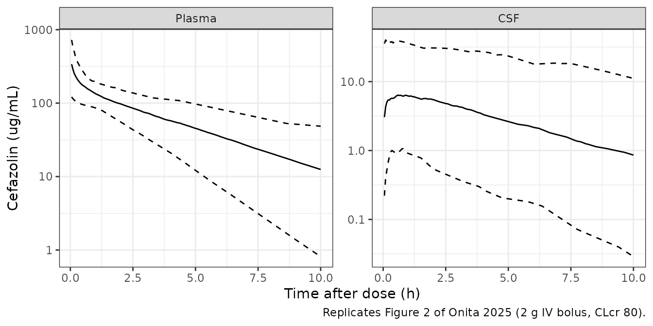
In the published figure the plasma median falls from about 380 ug/mL at time zero (2000 mg / 5.2 L) to about 8 ug/mL at 10 h, and the CSF median from about 6 to about 0.5 ug/mL. The simulated medians at 10 h are 12 (plasma) and 0.86 ug/mL (CSF), which is higher than the figure. The CSF-to-plasma ratio at 10 h is similar in both (about 0.07), so the difference is in plasma clearance. The paper does not say what renal function the VPC simulation assumed, and it does not report renal function for the patients behind the observed points (Supplementary Table S3, ‘NA’). At CLcr 80 the plasma model’s clearance is 2.86 L/h; a simulated cohort with better renal function would clear the drug faster and match the figure more closely. No parameter was adjusted.
Replicate Figure 3 and Table 1 (probability of target attainment)
cmin_csf <- sim |>
  group_by(arm, treatment, crcl, regimen, id) |>
  summarise(cmin = min(Ccsf), .groups = "drop")
pta <- cmin_csf |>
  tidyr::crossing(mic = mics) |>
  group_by(arm, treatment, crcl, regimen, mic) |>
  summarise(pta = 100 * mean(cmin > mic), .groups = "drop")

ggplot(pta |> filter(arm %in% regimens$arm[!is.na(regimens$bp_paper)]),
       aes(mic, pta, shape = regimen, colour = regimen)) +
  geom_line() +
  geom_point() +
  geom_hline(yintercept = 90, linetype = "dotted") +
  scale_x_log10(breaks = c(0.25, 1, 4, 16, 64), labels = c(0.25, 1, 4, 16, 64)) +
  scale_shape_manual(values = 0:14) +
  facet_wrap(~ factor(paste0("CLcr = ", crcl, " mL/min"), levels = paste0("CLcr = ", c(90, 60, 30), " mL/min")), ncol = 1) +
  labs(
    x = "MIC (ug/mL)", y = "PTA, 100% T > MIC in CSF (%)",
    shape = NULL, colour = NULL,
    caption = "Replicates Figure 3 of Onita 2025 (200 subjects per regimen)."
  ) +
  theme_bw() +
  theme(legend.position = "bottom") +
  guides(shape = guide_legend(ncol = 3), colour = guide_legend(ncol = 3))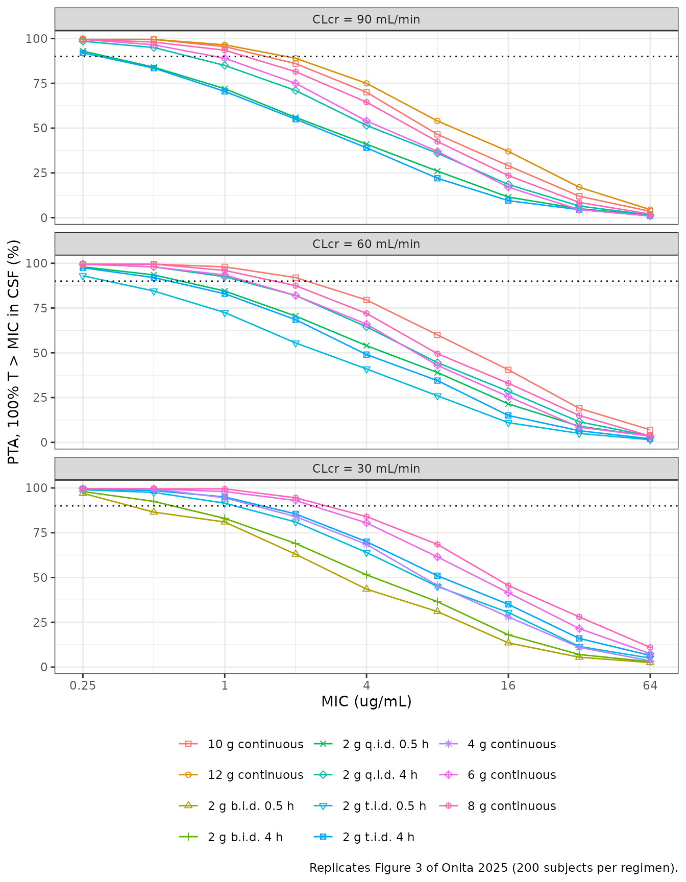
bp_sim <- pta |>
  group_by(arm) |>
  summarise(bp_sim = max(c(0, mic[pta >= 90])), .groups = "drop")
tab1 <- regimens |>
  filter(!is.na(bp_paper)) |>
  left_join(bp_sim, by = "arm")
n_exact <- sum(tab1$bp_sim == tab1$bp_paper)
# Common random numbers from base R make this deterministic; the paper's
# breakpoints come from its own 1000-subject Monte Carlo, so a regimen whose
# PTA sits near 90% at a breakpoint can land one dilution either side.
stopifnot(
  all(abs(log2(tab1$bp_sim / tab1$bp_paper)) <= 1),
  n_exact >= 18
)
knitr::kable(
  tab1 |>
    select(crcl, regimen, bp_paper, bp_sim) |>
    rename(
      "CLcr (mL/min)" = crcl, "Regimen" = regimen,
      "Table 1 breakpoint (ug/mL)" = bp_paper,
      "Simulated breakpoint (ug/mL)" = bp_sim
    ),
  caption = "PK/PD breakpoints (highest MIC with PTA of at least 90%), Table 1 of Onita 2025 against the simulation."
)| CLcr (mL/min) | Regimen | Table 1 breakpoint (ug/mL) | Simulated breakpoint (ug/mL) |
|---|---|---|---|
| 90 | 2 g q.i.d. 0.5 h | 0.25 | 0.25 |
| 90 | 2 g t.i.d. 4 h | 0.25 | 0.25 |
| 90 | 2 g q.i.d. 4 h | 0.50 | 0.50 |
| 90 | 6 g continuous | 0.50 | 0.50 |
| 90 | 8 g continuous | 1.00 | 1.00 |
| 90 | 10 g continuous | 1.00 | 1.00 |
| 90 | 12 g continuous | 1.00 | 1.00 |
| 60 | 2 g t.i.d. 0.5 h | 0.25 | 0.25 |
| 60 | 2 g q.i.d. 0.5 h | 0.50 | 0.50 |
| 60 | 2 g t.i.d. 4 h | 0.50 | 0.50 |
| 60 | 2 g q.i.d. 4 h | 1.00 | 1.00 |
| 60 | 6 g continuous | 1.00 | 1.00 |
| 60 | 8 g continuous | 1.00 | 1.00 |
| 60 | 10 g continuous | 2.00 | 2.00 |
| 30 | 2 g b.i.d. 0.5 h | 0.25 | 0.25 |
| 30 | 2 g t.i.d. 0.5 h | 1.00 | 1.00 |
| 30 | 2 g b.i.d. 4 h | 0.50 | 0.50 |
| 30 | 2 g t.i.d. 4 h | 2.00 | 1.00 |
| 30 | 4 g continuous | 1.00 | 1.00 |
| 30 | 6 g continuous | 2.00 | 2.00 |
| 30 | 8 g continuous | 2.00 | 2.00 |
20 of 21 simulated breakpoints equal Table 1, and the rest are within one doubling dilution.
Replicate Supplementary Table S2 (neurotoxicity exceedance)
s2_paper <- tibble::tribble(
  ~treatment,                   ~p64_paper,
  "CLcr 90: 2 g q.i.d. 0.5 h",  1.1,
  "CLcr 90: 2 g t.i.d. 4 h",    0.8,
  "CLcr 90: 2 g q.i.d. 4 h",    1.8,
  "CLcr 60: 2 g t.i.d. 0.5 h",  1.0,
  "CLcr 60: 2 g q.i.d. 0.5 h",  2.3,
  "CLcr 60: 2 g t.i.d. 4 h",    1.6,
  "CLcr 60: 2 g q.i.d. 4 h",    3.0,
  "CLcr 30: 2 g b.i.d. 0.5 h",  1.1,
  "CLcr 30: 2 g t.i.d. 0.5 h",  3.7,
  "CLcr 30: 2 g b.i.d. 4 h",    1.8,
  "CLcr 30: 2 g t.i.d. 4 h",    9.0
) |>
  bind_rows(s2_ci)
s2_sim <- cmin_csf |>
  group_by(treatment) |>
  summarise(p64_sim = 100 * mean(cmin > 64), .groups = "drop") |>
  inner_join(s2_paper, by = "treatment")
stopifnot(
  nrow(s2_sim) == 21,
  median(abs(s2_sim$p64_sim - s2_sim$p64_paper)) < 1.5,
  quantile(abs(s2_sim$p64_sim - s2_sim$p64_paper), 0.9) < 3
)
knitr::kable(
  s2_sim |>
    rename(
      "Regimen" = treatment, "Simulated (%)" = p64_sim,
      "Table S2 (%)" = p64_paper
    ),
  digits = 1,
  caption = "Probability that the steady-state CSF trough exceeds 64 ug/mL."
)| Regimen | Simulated (%) | Table S2 (%) |
|---|---|---|
| CLcr 30: 2 g b.i.d. 0.5 h | 2.5 | 1.1 |
| CLcr 30: 2 g b.i.d. 4 h | 3.0 | 1.8 |
| CLcr 30: 2 g t.i.d. 0.5 h | 5.0 | 3.7 |
| CLcr 30: 2 g t.i.d. 4 h | 6.5 | 9.0 |
| CLcr 30: 4 g continuous | 3.5 | 3.5 |
| CLcr 30: 6 g continuous | 7.5 | 6.6 |
| CLcr 30: 8 g continuous | 11.0 | 9.9 |
| CLcr 60: 10 g continuous | 7.0 | 6.1 |
| CLcr 60: 2 g q.i.d. 0.5 h | 3.5 | 2.3 |
| CLcr 60: 2 g q.i.d. 4 h | 3.5 | 3.0 |
| CLcr 60: 2 g t.i.d. 0.5 h | 1.5 | 1.0 |
| CLcr 60: 2 g t.i.d. 4 h | 2.0 | 1.6 |
| CLcr 60: 6 g continuous | 3.5 | 2.6 |
| CLcr 60: 8 g continuous | 3.5 | 4.3 |
| CLcr 90: 10 g continuous | 3.5 | 4.0 |
| CLcr 90: 12 g continuous | 4.5 | 5.0 |
| CLcr 90: 2 g q.i.d. 0.5 h | 1.5 | 1.1 |
| CLcr 90: 2 g q.i.d. 4 h | 1.5 | 1.8 |
| CLcr 90: 2 g t.i.d. 4 h | 1.0 | 0.8 |
| CLcr 90: 6 g continuous | 1.0 | 1.4 |
| CLcr 90: 8 g continuous | 2.0 | 2.5 |
With 200 subjects one subject is 0.5 percentage points, so the simulated exceedances agree with Table S2 to within Monte Carlo error.
PKNCA validation
NCA over one steady-state dosing interval, in plasma and CSF, for the
CLcr 90 mL/min regimens used in the paper’s external comparison
(Supplementary Table S1). Because the CSF compartment’s inflow and
outflow are both proportional to the CSF flow, integrating the CSF
equation over a steady-state interval gives
AUC_csf = kp_csf x AUC_plasma for every subject, whatever
its CSF flow and volume. The per-subject AUC ratio is checked against
kp_csf.
nca_arms <- regimens$arm[regimens$treatment %in% c(
  "CLcr 90: 2 g t.i.d. 0.5 h", "CLcr 90: 2 g t.i.d. 4 h",
  "CLcr 90: 8 g continuous"
)]
nca_conc <- sim |>
  filter(arm %in% nca_arms) |>
  # 0.25 h subsample keeps the NCA fast; it includes every dosing-interval
  # boundary.
  filter(abs(time / 0.25 - round(time / 0.25)) < 1e-8) |>
  select(id, time, treatment, tau, Plasma = Cc, CSF = Ccsf) |>
  pivot_longer(c(Plasma, CSF), names_to = "matrix", values_to = "Cc") |>
  filter(!is.na(Cc))
nca_dose <- events |>
  filter(evid == 1, arm %in% nca_arms) |>
  left_join(regimens |> select(arm, treatment), by = "arm") |>
  select(id, time, amt, treatment)

conc_obj <- PKNCA::PKNCAconc(nca_conc, Cc ~ time | treatment + matrix + id)
dose_obj <- PKNCA::PKNCAdose(nca_dose, amt ~ time | treatment + id)
intervals <- regimens |>
  filter(arm %in% nca_arms) |>
  transmute(
    treatment, start = 0, end = tau,
    cmax = TRUE, cmin = TRUE, cav = TRUE, auclast = TRUE
  )
nca_res <- PKNCA::pk.nca(
  PKNCA::PKNCAdata(
    conc_obj, dose_obj,
    intervals = intervals,
    # Linear trapezoids: log-down interpolation is biased on the nearly flat
    # continuous-infusion profiles.
    options = list(auc.method = "linear")
  )
)
nca_tab <- as.data.frame(nca_res$result)

auc_ratio <- nca_tab |>
  filter(PPTESTCD == "auclast") |>
  select(treatment, matrix, id, PPORRES) |>
  pivot_wider(names_from = matrix, values_from = PPORRES) |>
  left_join(sim |> distinct(id, kp_csf), by = "id") |>
  mutate(rel = CSF / Plasma / kp_csf)
stopifnot(
  nrow(auc_ratio) == length(nca_arms) * N_SUBJ,
  abs(median(auc_ratio$rel) - 1) < 0.01,
  quantile(abs(auc_ratio$rel - 1), 0.9) < 0.03
)

knitr::kable(
  nca_tab |>
    filter(PPTESTCD %in% c("cmax", "cmin", "cav")) |>
    group_by(treatment, matrix, PPTESTCD) |>
    summarise(median = median(PPORRES), .groups = "drop") |>
    mutate(PPTESTCD = ncaParamLabel(PPTESTCD)) |>
    pivot_wider(names_from = PPTESTCD, values_from = median) |>
    rename("Regimen" = treatment, "Matrix" = matrix),
  digits = 2,
  caption = "Median steady-state NCA (ug/mL), CLcr 90 mL/min."
)| Regimen | Matrix | Cavg | Cmax | Cmin |
|---|---|---|---|---|
| CLcr 90: 2 g t.i.d. 0.5 h | CSF | 4.35 | 10.25 | 1.45 |
| CLcr 90: 2 g t.i.d. 0.5 h | Plasma | 79.94 | 257.49 | 20.56 |
| CLcr 90: 2 g t.i.d. 4 h | CSF | 4.35 | 6.65 | 2.35 |
| CLcr 90: 2 g t.i.d. 4 h | Plasma | 79.94 | 123.51 | 35.08 |
| CLcr 90: 8 g continuous | CSF | 5.80 | 5.80 | 5.80 |
| CLcr 90: 8 g continuous | Plasma | 106.59 | 106.59 | 106.59 |
Comparison against published values
Supplementary Table S1 reports the paper’s own simulated median CSF concentration for two regimens at CLcr 90 mL/min: 5.7 ug/mL for 8 g/day by continuous infusion and a 1.2 ug/mL trough for 2 g three times daily. The infusion duration of the 2 g t.i.d. regimen is not stated, so both 0.5 h and 4 h are shown.
nca_ref <- data.frame(
  treatment = c(
    "CLcr 90: 8 g continuous", "CLcr 90: 2 g t.i.d. 0.5 h",
    "CLcr 90: 2 g t.i.d. 4 h"
  ),
  cav = c(5.7, NA, NA),
  cmin = c(NA, 1.2, 1.2)
)
nca_csf <- nca_tab |> filter(matrix == "CSF")
# One call per parameter, each restricted to the regimens that have a
# published reference value for it.
cmp <- bind_rows(
  ncaComparisonTable(
    simulated = nca_csf |> filter(treatment == "CLcr 90: 8 g continuous"),
    reference = nca_ref |> filter(!is.na(cav)) |> select(treatment, cav),
    by = "treatment", params = "cav", units = c(cav = "ug/mL")
  ),
  ncaComparisonTable(
    simulated = nca_csf |> filter(treatment != "CLcr 90: 8 g continuous"),
    reference = nca_ref |> filter(!is.na(cmin)) |> select(treatment, cmin),
    by = "treatment", params = "cmin", units = c(cmin = "ug/mL")
  )
)
knitr::kable(cmp, caption = "Median CSF concentrations: Onita 2025 Supplementary Table S1 against this implementation.")| NCA parameter | treatment | Reference | Simulated | % diff |
|---|---|---|---|---|
| Cavg (ug/mL) | CLcr 90: 8 g continuous | 5.7 | 5.8 | +1.7% |
| Cmin (ug/mL) | CLcr 90: 2 g t.i.d. 0.5 h | 1.2 | 1.45 | +20.9%* |
| Cmin (ug/mL) | CLcr 90: 2 g t.i.d. 4 h | 1.2 | 2.35 | +96.0%* |
cmp_num <- nca_tab |>
  filter(matrix == "CSF", treatment == "CLcr 90: 8 g continuous", PPTESTCD == "cav")
# 200 subjects with a log-scale SD of 1.22 gives the median about 11% Monte
# Carlo error.
stopifnot(abs(median(cmp_num$PPORRES) / 5.7 - 1) < 0.25)
The 8 g/day median matches. For the 2 g t.i.d. trough, the paper’s 1.2 ug/mL is closer to the 0.5 h infusion than to the 4 h infusion. The remaining difference from the 0.5 h value is within the Monte Carlo error of a 200-subject median at this level of variability. The measured values the paper compares against were 6.1 ug/mL (one case report, 8 g/day continuous), a median of 2.8 ug/mL (range 2.1-5.2; 8 g/day, mainly continuous) and a median trough of 1.59 ug/mL (range 0.7-2.2; 2 g t.i.d.), in patients with normal renal function.
Assumptions and deviations
- Hybrid model, not a fit. All structural values are literature values held constant (Table 2 footnotes a-c). Only the CSF variances were estimated, from 24 CSF samples in 8 patients. The RSEs of 0.75% and 0.38% on the CSF flow and volume variances, next to a sampling-importance-resampling interval spanning five orders of magnitude, show that these variances are poorly identified. They are carried as published.
-
No CL-Vc correlation. Lanoiselee 2021 estimated a
CL-Vc correlation of 0.83. Onita 2025 Table 2 lists only the diagonal
variances, so the omega matrix here is diagonal. At steady state under
continuous infusion
Vcdoes not affect the CSF concentration, so the continuous-infusion results above do not depend on this choice. -
CSF compartment is a satellite. The Methods 4.1
equations do not remove the CSF inflow from
centralor return the CSF outflow to it. The equations are encoded as printed. The CSF flow (0.021 L/h) is under 1% of the clearance, so the effect on plasma mass balance is negligible. -
Single residual error for both matrices. Table 2
lists one proportional epsilon (variance 0.0144). nlmixr2 needs one
residual parameter per endpoint, so
propSdandpropSd_Ccsfboth carry 0.12. -
Renal function units. The paper writes CLcr in
mL/min and simulates at 90, 60 and 30 mL/min. The covariate is the
CKD-EPI estimate the plasma model was built on, recorded in its native
mL/min/1.73 m^2 as in
Lanoiselee_2021_cefazolin. Simulations here use the paper’s numbers unchanged. - Figure 2 conditions. The figure gives neither the creatinine clearance nor the dose route of the normalised profiles. A 2 g bolus at CLcr 80 (the plasma model’s reference) was used, which matches the plasma median of about 380 ug/mL at time zero.
- Cohort size. The paper simulated 1000 subjects per regimen; 200 common random-number subjects are used here. Breakpoints whose PTA sits near 90% can differ by one dilution (one of 21 regimens here).
- Total concentration. The paper does not correct CSF concentrations for protein binding, and neither does this model.