Lacosamide time-to-seizure and dropout (Lindauer 2017)
Source:vignettes/articles/Lindauer_2017_lacosamide.Rmd
Lindauer_2017_lacosamide.RmdModel and source
- Citation: Lindauer A, Laveille C, Stockis A. Time-to-seizure modeling of lacosamide used in monotherapy in patients with newly diagnosed epilepsy. Clin Pharmacokinet. 2017;56(11):1403-1413. doi:10.1007/s40262-017-0530-8.
- Article: https://doi.org/10.1007/s40262-017-0530-8 (Open Access under CC BY-NC 4.0)
- Sister model files (one paper, two independent time-to-event
sub-models):
-
modellib("Lindauer_2017_lacosamide_dropout")– dropout hazard (dropout not because of a lack of efficacy). -
modellib("Lindauer_2017_lacosamide_seizure")– repeated time-to-seizure hazard with distinct first-seizure and 2nd-and-subsequent-seizure Weibull sub-models.
-
Population
Data came from the SP0993 trial (ClinicalTrials.gov identifier NCT01243177), a multicenter, double-blind, double-dummy, randomized, positive-controlled, non-inferiority trial comparing lacosamide (LCM) and carbamazepine controlled-release (CBZ-CR) monotherapy in adult patients newly diagnosed with focal or generalized tonic-clonic seizures without signs of focal onset (idiopathic generalized epilepsy history was an exclusion). Of 888 randomized patients, 883 (LCM 443, CBZ-CR 440) were analyzed. Median age 40 years (range 16-87, IQR 26-55); 46.3% female. Median number of seizures in the previous 3 months (NSP3M) was 2 (range 0-450, IQR 1-6). LCM target dose levels were 200, 400, or 600 mg/day BID (starting dose 100 mg/day); CBZ-CR target dose levels were 400, 800, or 1200 mg/day BID (starting dose 200 mg/day). Dose escalation to the next level was triggered by seizure occurrence during the 26-week evaluation period at the current dose. Baseline demographics are in Lindauer 2017 Table 1.
The population metadata is available programmatically:
readModelDb("Lindauer_2017_lacosamide_seizure")()$population
#> $species
#> [1] "human"
#>
#> $n_subjects
#> [1] 883
#>
#> $n_studies
#> [1] 1
#>
#> $age_range
#> [1] "16-87 years (median 40, IQR 26-55)"
#>
#> $weight_range
#> [1] "not reported in the paper"
#>
#> $sex_female_pct
#> [1] 46.3
#>
#> $race_ethnicity
#> NULL
#>
#> $disease_state
#> [1] "Adult patients (>=16 years) newly diagnosed with focal or generalized tonic-clonic seizures without signs of focal onset, provided they had no history or clinical or electroencephalographic findings suggestive of idiopathic generalized epilepsy (SP0993 inclusion criteria; ClinicalTrials.gov NCT01243177)."
#>
#> $dose_range
#> [1] "LCM target dose levels 200, 400, or 600 mg/day BID (randomisation starting dose 100 mg/day); CBZ-CR target dose levels 400, 800, or 1200 mg/day BID (randomisation starting dose 200 mg/day). Dose escalation to the next level was triggered by seizure occurrence during the 26-week evaluation period at the current dose."
#>
#> $regions
#> [1] "multinational (SP0993)"
#>
#> $biomarkers
#> [1] "Repeated time-to-seizure (seizure defined as one seizure-event day, so multiple seizures on the same day count as a single event). About 55% of patients had no seizures during the trial; 15% had one seizure; about 30% had two or more (Lindauer 2017 Section 3.1). Baseline covariate NSP3M (seizure count in the previous 3 months) had median 2 and range 0-450."
#>
#> $notes
#> [1] "Randomised 883 patients (LCM 443, CBZ-CR 440) analysed for seizures. Seizure model was originally developed on the historic N01061 dataset (comparing levetiracetam and CBZ-CR; NCT00150735) using the two-Weibull-sub-model approach of Abrantes et al. and re-estimated on SP0993 as described in Lindauer 2017 Section 2.2 'Modeling Strategy and Software'."
Source trace
The parameter provenance is recorded as an in-file comment next to
each ini() entry in the two model files. This table
collects the primary values in one place.
Dropout model (Lindauer 2017 Table 2)
| Parameter (canonical) | Value | Source location |
|---|---|---|
bp1_drop (log breakpoint 1) |
log(20) |
Table 2 BP1 = 20 d |
dbp2_drop (log delta BP2-BP1) |
log(9.76) |
Table 2 D(BP2-BP1) = 9.76 d |
dbp3_drop (log delta BP3-BP2) |
log(105) |
Table 2 D(BP3-BP2) = 105 d |
dbp4_drop (log delta BP4-BP3) |
log(340) |
Table 2 D(BP4-BP3) = 340 d |
lk1_drop |
log(0.00205) |
Table 2 k1 = 0.00205 /day |
lk2_drop |
log(0.00358) |
Table 2 k2 = 0.00358 /day |
lk3_drop |
log(0.000946) |
Table 2 k3 = 0.000946 /day |
lk4_drop |
log(0.000613) |
Table 2 k4 = 0.000613 /day |
lk5_drop |
log(0.00221) |
Table 2 k5 = 0.00221 /day |
e_sexf_drop |
0.238 |
Table 2 Coeff_SEX (HR_SEX = 1.27) |
e_conmed_lcm_drop |
-0.138 |
Table 2 Coeff_TYPE (HR_TYPE = 0.871) |
Smoothing steepness gam
|
50 (hardcoded) |
Section 2.4 narrative “a high value of 50 was chosen for the GAM variable” |
Sigmoid form
s_i = 1 / (1 + exp(-gam * (t - bp_i)))
|
– | Section 2.4 Frobel et al. reference |
Seizure model (Lindauer 2017 Table 3)
Weibull baseline hazard
h(t) = lam * p * (lam * t)^(p - 1); log-linear covariate
effects on ln(lam); the paper’s Table 4 hazard ratios are
derived via HR = exp(coefficient * p) for continuous
covariates (with p = p1 for first-seizure and p2 for
subsequent-seizure sub-models).
| Parameter (canonical) | Value | Source location |
|---|---|---|
llam_1st |
log(0.000733) |
Table 3 k1 = 0.000733 /day |
lp_1st |
log(0.493) |
Table 3 p1 = 0.493 |
llam_2nd |
log(0.00889) |
Table 3 k2 = 0.00889 /day |
lp_2nd |
log(0.713) |
Table 3 p2 = 0.713 |
e_nsp3m_lt2_1st |
-1.12 |
Table 3 NSP3M(<2)*k1 (HR = 0.58 per Table 4) |
e_nsp3m_7_50_1st |
+1.94 |
Table 3 NSP3M(7-50)*k1 (HR = 2.60 per Table 4) |
e_nsp3m_gt50_1st |
+3.30 |
Table 3 NSP3M(>50)*k1 (HR = 5.09 per Table 4) |
e_nsp3m_lt2_2nd |
-1.37 |
Table 3 NSP3M(<2)*k2 (HR = 0.38 per Table 4) |
e_nsp3m_7_50_2nd |
+1.36 |
Table 3 NSP3M(7-50)*k2 (HR = 2.63 per Table 4) |
e_nsp3m_gt50_2nd |
+2.53 |
Table 3 NSP3M(>50)*k2 (HR = 6.09 per Table 4) |
e_auc_lcm_1st |
-0.00917 |
Table 3 AUC_LCM*k1 |
e_auc_cbz_1st |
-0.00658 |
Table 3 AUC_CBZ*k1 |
e_auc_lcm_2nd |
-0.00751 |
Table 3 AUC_LCM*k2 |
e_auc_cbz_2nd |
-0.0153 |
Table 3 AUC_CBZ*k2 |
e_age_1st |
-0.0256 |
Table 3 AGE*k1 (LCM only; HR AGE 65 vs 41 = 0.74 per Table 4) |
etallam_2nd variance |
2.03^2 = 4.1209 |
Table 3 IIV ln(k2) SD = 2.03 |
| AUC reference LCM | 104 mg*h/L |
Table 3 note c (“AUC centered on typical value at the first dose level” = 200 mg/day LCM) |
| AUC reference CBZ | 132 mg*h/L |
Section 3.4 first paragraph (“typical CBZ AUC of 132 mg*h/L … 70-kg patient receiving CBZ-CR 400 mg/day”) |
| AGE reference | 41 years |
Table 3 note d (“AGE centered on 41 years”) + Table 1 cohort median |
Hazard-ratio spot check
The Weibull-shape multiplier is worth verifying explicitly because it is easy to mistranslate:
# NSP3M 7-50 vs 2-6 first seizure: Table 4 reports HR = 2.60
# HR = exp(coef * p1) = exp(1.94 * 0.493) = 2.605
p1 <- 0.493
p2 <- 0.713
exp(c(nsp3m_7_50_1st = 1.94 * p1,        # ~ log(2.60)
      nsp3m_gt50_1st = 3.30 * p1,        # ~ log(5.09)
      auc_lcm_300_vs_100_1st = -0.00917 * 200 * p1, # ~ log(0.40)
      age_65_vs_41_1st = -0.0256 * 24 * p1))         # ~ log(0.74)
#>         nsp3m_7_50_1st         nsp3m_gt50_1st auc_lcm_300_vs_100_1st
#>              2.6023633              5.0880772              0.4048810
#>       age_65_vs_41_1st
#>              0.7386736
The values reproduce Table 4 to two decimal places.
Virtual cohort
Original observed data are not publicly available. The simulations below use virtual cohorts sized to reproduce the paper’s typical-value hazard curves and the SP0993 arm structure. Cohorts are capped at 200 subjects per arm per the project convention.
The event table below builds one cohort of 200 LCM-arm patients and 200 CBZ-CR patients with all subjects observed nightly (once per day) from day 0 to day 385 (21 days up-titration/stabilization + 364 days at maintenance dose without escalation, per Lindauer 2017 Section 3.4). Baseline covariates are drawn to match the SP0993 marginal demographics (Table 1).
set.seed(42)

n_per_arm <- 60L
sim_days  <- 385L
obs_times <- c(seq(0, 30, by = 3), seq(35, sim_days, by = 7))

# Baseline NSP3M distribution from Table 1 (Total column).
nsp3m_probs <- c(lt2 = 0.257, ref_2_6 = 0.514, m_7_50 = 0.181, gt50 = 0.048)

make_arm <- function(n, arm_label, id_offset = 0L) {
  arm_is_lcm <- as.integer(arm_label == "LCM")
  # LCM at 200 mg/day gives AUC ~ 104 mg*h/L; CBZ-CR at 400 mg/day gives ~ 132
  # mg*h/L. Simulation is at the reference (first) dose level so covariate
  # AUC values equal the paper's centring anchors and the AUC contribution
  # to the hazard is zero.
  auc_lcm <- if (arm_is_lcm) 104 else 0
  auc_cbz <- if (arm_is_lcm) 0   else 132
  # Baseline covariates
  nsp3m_cat <- sample(names(nsp3m_probs), size = n, replace = TRUE,
                      prob = nsp3m_probs)
  tibble::tibble(
    id        = id_offset + seq_len(n),
    arm       = arm_label,
    AGE       = round(rnorm(n, mean = 41, sd = 15)),
    SEXF      = rbinom(n, 1, 0.463),
    CONMED_LCM = arm_is_lcm,
    NSP3M_LT2  = as.integer(nsp3m_cat == "lt2"),
    NSP3M_7_50 = as.integer(nsp3m_cat == "m_7_50"),
    NSP3M_GT50 = as.integer(nsp3m_cat == "gt50"),
    AUC_LCM   = auc_lcm,
    AUC_CBZ   = auc_cbz
  ) |>
    # Truncate ages to the reported inclusion range 16-87 years
    dplyr::mutate(AGE = pmin(pmax(AGE, 16L), 87L))
}

subjects <- dplyr::bind_rows(
  make_arm(n_per_arm, "LCM",   id_offset = 0L),
  make_arm(n_per_arm, "CBZ-CR", id_offset = n_per_arm)
)

# One observation row per subject at obs_times; time in days.
events <- subjects |>
  tidyr::crossing(time = obs_times) |>
  dplyr::mutate(
    evid = 0L,
    amt  = 0,
    cmt  = "cumhaz_drop"        # a state name; the actual state depends on model
  ) |>
  dplyr::arrange(id, time)

# rxSolve accepts a data-frame event table with covariates. Convert to the
# format expected by rxode2's rxSolve() -- an ordinary tibble is fine here
# because there are no dosing events (evid = 0 throughout).
head(events, 5)
#> # A tibble: 5 × 14
#>      id arm     AGE  SEXF CONMED_LCM NSP3M_LT2 NSP3M_7_50 NSP3M_GT50 AUC_LCM
#>   <int> <chr> <dbl> <int>      <int>     <int>      <int>      <int>   <dbl>
#> 1     1 LCM      48     1          1         0          1          0     104
#> 2     1 LCM      48     1          1         0          1          0     104
#> 3     1 LCM      48     1          1         0          1          0     104
#> 4     1 LCM      48     1          1         0          1          0     104
#> 5     1 LCM      48     1          1         0          1          0     104
#> # ℹ 5 more variables: AUC_CBZ <dbl>, time <dbl>, evid <int>, amt <dbl>,
#> #   cmt <chr>
Simulation – dropout model
The dropout hazard depends on time (via the 4-breakpoint smoothed
step function) and on SEXF + CONMED_LCM. IIV
is not modelled (Lindauer 2017 Table 2 reports no eta on the dropout
hazard); the simulation therefore returns a typical-value trajectory per
(SEXF, CONMED_LCM) combination.
mod_drop <- readModelDb("Lindauer_2017_lacosamide_dropout")

sim_drop <- rxode2::rxSolve(
  mod_drop,
  events = events,
  keep = c("arm", "SEXF", "CONMED_LCM")
)
#> Warning: multi-subject simulation without without 'omega'

head(sim_drop, 5)
#>   id time bp1   bp2    bp3    bp4      k1      k2       k3       k4      k5
#> 1  1    0  20 29.76 134.76 474.76 0.00205 0.00358 0.000946 0.000613 0.00221
#> 2  1    3  20 29.76 134.76 474.76 0.00205 0.00358 0.000946 0.000613 0.00221
#> 3  1    6  20 29.76 134.76 474.76 0.00205 0.00358 0.000946 0.000613 0.00221
#> 4  1    9  20 29.76 134.76 474.76 0.00205 0.00358 0.000946 0.000613 0.00221
#> 5  1   12  20 29.76 134.76 474.76 0.00205 0.00358 0.000946 0.000613 0.00221
#>              s1 s2 s3 s4 h0_drop hazard_drop       sur  ipredSim       sim
#> 1  0.000000e+00  0  0  0 0.00205   0.0022656 1.0000000 1.0000000 0.9987947
#> 2  0.000000e+00  0  0  0 0.00205   0.0022656 0.9932262 0.9932262 0.9944859
#> 3 9.859677e-305  0  0  0 0.00205   0.0022656 0.9864984 0.9864984 0.9861204
#> 4 1.374153e-239  0  0  0 0.00205   0.0022656 0.9798161 0.9798161 0.9793847
#> 5 1.915170e-174  0  0  0 0.00205   0.0022656 0.9731790 0.9731790 0.9724372
#>   cumhaz_drop SEXF CONMED_LCM arm
#> 1 0.000000000    1          1 LCM
#> 2 0.006796801    1          1 LCM
#> 3 0.013593602    1          1 LCM
#> 4 0.020390403    1          1 LCM
#> 5 0.027187205    1          1 LCM
Figure 2 – Replicate KM VPC of dropout by arm
Lindauer 2017 Figure 2 shows the observed and predicted dropout
Kaplan-Meier curves. Here we plot the model’s typical-value dropout-free
survival (sur = exp(-cumhaz_drop)) by treatment arm and
overlay the paper’s reported hazard ratio for LCM vs CBZ-CR.
sim_drop |>
  dplyr::group_by(time, arm) |>
  dplyr::summarise(mean_sur = mean(sur), .groups = "drop") |>
  ggplot(aes(time, mean_sur, colour = arm)) +
  geom_line(linewidth = 0.8) +
  scale_y_continuous(limits = c(0, 1), breaks = seq(0, 1, 0.2)) +
  labs(x = "Time (days)", y = "Dropout-free survival probability",
       colour = "Arm",
       title = "Figure 2 -- Dropout-free survival by arm",
       caption = "Replicates the shape of Fig. 2 (Lindauer 2017); LCM-vs-CBZ-CR HR = 0.871.")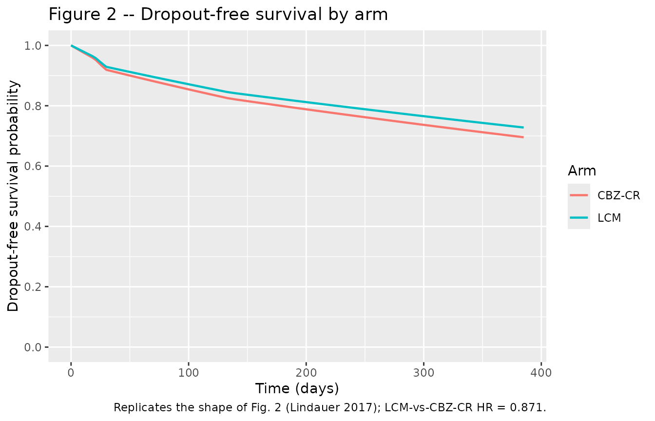
The paper’s Discussion Section 4.1 quotes a hazard ratio of 0.871 (90% CI 0.714-1.06) for LCM vs CBZ-CR; the simulated curves show LCM slightly above CBZ-CR consistent with a modestly protective LCM effect.
Female-vs-male:
sim_drop |>
  dplyr::group_by(time, SEXF) |>
  dplyr::summarise(mean_sur = mean(sur), .groups = "drop") |>
  dplyr::mutate(sex = ifelse(SEXF == 1, "Female", "Male")) |>
  ggplot(aes(time, mean_sur, colour = sex)) +
  geom_line(linewidth = 0.8) +
  scale_y_continuous(limits = c(0, 1), breaks = seq(0, 1, 0.2)) +
  labs(x = "Time (days)", y = "Dropout-free survival probability",
       colour = "Sex",
       title = "Dropout-free survival by sex",
       caption = "HR_SEX = 1.27 (Lindauer 2017 Table 2): females have a higher dropout hazard.")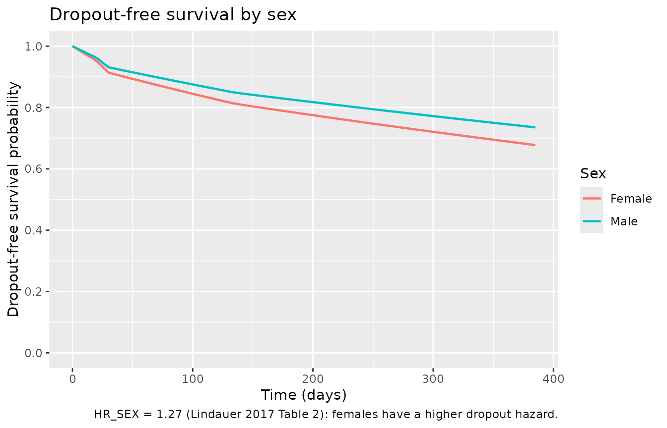
Simulation – seizure model
The seizure model has two Weibull sub-models. The primary observation
sur is the first-seizure survivor function; the derived
output sur_2nd is the subsequent-seizure survivor function
(integrated from t = 0 for diagnostic comparison). NSP3M
category is the dominant covariate.
mod_seiz <- readModelDb("Lindauer_2017_lacosamide_seizure")

# The 2nd+ hazard carries an eta with SD 2.03 on ln(lam). Zero the random
# effects for the typical-value replication.
mod_seiz_typical <- rxode2::zeroRe(mod_seiz)
#> ℹ parameter labels from comments will be replaced by 'label()'

sim_seiz_typical <- rxode2::rxSolve(
  mod_seiz_typical,
  events = events,
  keep = c("arm", "CONMED_LCM", "AGE", "NSP3M_LT2", "NSP3M_7_50", "NSP3M_GT50")
)
#> ℹ omega/sigma items treated as zero: 'etallam_2nd'
#> Warning: multi-subject simulation without without 'omega'

head(sim_seiz_typical, 5)
#>   id time lam1_typical    p1 lam2_typical    p2 cov_nsp3m_1st cov_nsp3m_2nd
#> 1  1    0     0.000733 0.493      0.00889 0.713          1.94          1.36
#> 2  1    3     0.000733 0.493      0.00889 0.713          1.94          1.36
#> 3  1    6     0.000733 0.493      0.00889 0.713          1.94          1.36
#> 4  1    9     0.000733 0.493      0.00889 0.713          1.94          1.36
#> 5  1   12     0.000733 0.493      0.00889 0.713          1.94          1.36
#>   cov_auc_1st cov_auc_2nd cov_age_1st    lam1_eff   lam2_eff   hazard_1st
#> 1           0           0     -0.1792 0.004263926 0.03463716 36.841991717
#> 2           0           0     -0.1792 0.004263926 0.03463716  0.019162076
#> 3           0           0     -0.1792 0.004263926 0.03463716  0.013484051
#> 4           0           0     -0.1792 0.004263926 0.03463716  0.010978478
#> 5           0           0     -0.1792 0.004263926 0.03463716  0.009488514
#>   hazard_2nd       sur   sur_2nd  ipredSim       sim cumhaz_1st cumhaz_2nd AGE
#> 1 3.41808736 1.0000000 1.0000000 1.0000000 1.0000000  0.0000000  0.0000000  48
#> 2 0.04729871 0.8900027 0.8195429 0.8900027 0.8900027  0.1165308  0.1990085  48
#> 3 0.03876624 0.8487147 0.7216467 0.8487147 0.8487147  0.1640322  0.3262196  48
#> 4 0.03450766 0.8184485 0.6468915 0.8184485 0.8184485  0.2003448  0.4355767  48
#> 5 0.03177299 0.7938314 0.5858186 0.7938314 0.7938314  0.2308842  0.5347452  48
#>   CONMED_LCM NSP3M_LT2 NSP3M_7_50 NSP3M_GT50 AUC_LCM AUC_CBZ arm
#> 1          1         0          1          0     104       0 LCM
#> 2          1         0          1          0     104       0 LCM
#> 3          1         0          1          0     104       0 LCM
#> 4          1         0          1          0     104       0 LCM
#> 5          1         0          1          0     104       0 LCM
Figure 3 – Replicate KM VPC of time to first seizure by baseline severity
Lindauer 2017 Figure 3 shows the time-to-first-seizure Kaplan-Meier
curve in the evaluation phase (t >= 21 days after the up-titration /
stabilization). Here we plot the typical-value first-seizure survivor
function sur stratified by NSP3M category to highlight the
dominant baseline-severity effect. Curves correspond to the paper’s
Table 4 first-seizure hazard-ratio comparisons (NSP3M_LT2 vs. reference
vs. 7-50 vs. >50).
sim_seiz_typical |>
  dplyr::mutate(nsp3m_cat = dplyr::case_when(
    NSP3M_LT2  == 1 ~ "<2",
    NSP3M_7_50 == 1 ~ "7-50",
    NSP3M_GT50 == 1 ~ ">50",
    TRUE            ~ "2-6 (ref)"
  )) |>
  dplyr::group_by(time, nsp3m_cat, arm) |>
  dplyr::summarise(mean_sur = mean(sur), .groups = "drop") |>
  ggplot(aes(time, mean_sur, colour = nsp3m_cat)) +
  geom_line(linewidth = 0.7) +
  facet_wrap(~arm) +
  scale_y_continuous(limits = c(0, 1), breaks = seq(0, 1, 0.2)) +
  labs(x = "Time (days)", y = "First-seizure-free survival probability",
       colour = "NSP3M category",
       title = "Figure 3 -- First-seizure-free survival by baseline seizure severity",
       caption = "Table 4 first-seizure HRs vs 2-6: <2 HR 0.58; 7-50 HR 2.60; >50 HR 5.09.")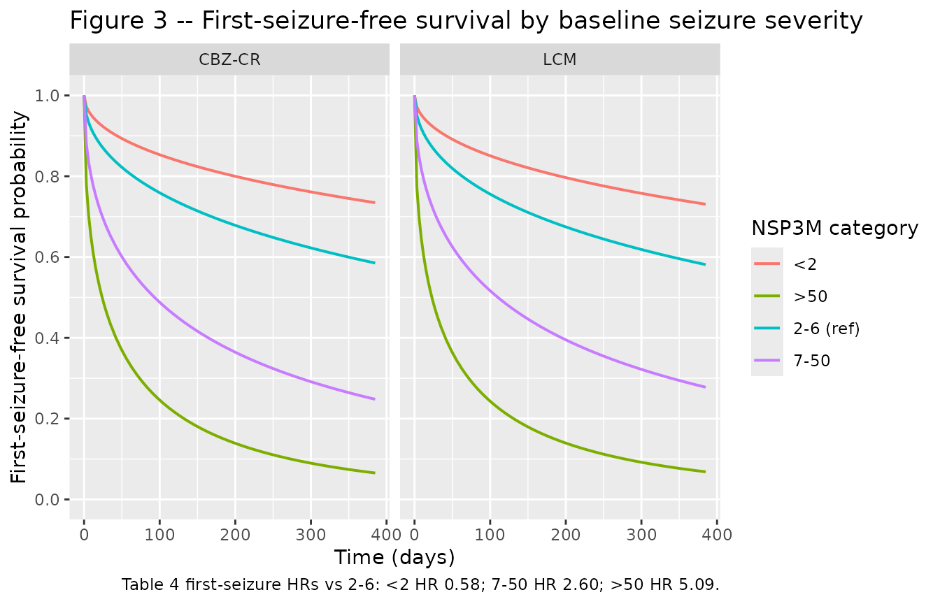
The stratification reproduces the dominant NSP3M effect described in the paper Abstract: patients with 7-50 baseline seizures have a 2.6-fold higher seizure hazard than the 2-6 reference, and >50 patients show a further substantial elevation.
AGE effect on the LCM arm (first-seizure sub-model only)
Lindauer 2017 Results Section 3.4 states that a significant AGE effect on first-seizure hazard was identified only in the LCM arm (“indicating a treatment-age interaction”), with HR = 0.74 for AGE 65 vs 41 years.
# Synthetic age contrast: 41-year-old and 65-year-old patients, LCM arm,
# NSP3M reference category (2-6). Take typical-value trajectories.
age_events <- tibble::tibble(
  id = 1:2, AGE = c(41L, 65L), SEXF = 0L,
  CONMED_LCM = 1L, NSP3M_LT2 = 0L, NSP3M_7_50 = 0L, NSP3M_GT50 = 0L,
  AUC_LCM = 104, AUC_CBZ = 0
) |>
  tidyr::crossing(time = obs_times) |>
  dplyr::mutate(evid = 0L, amt = 0)

sim_age <- rxode2::rxSolve(mod_seiz_typical, events = age_events,
                           keep = c("AGE"))
#> ℹ omega/sigma items treated as zero: 'etallam_2nd'
#> Warning: multi-subject simulation without without 'omega'
sim_age |>
  dplyr::group_by(time, AGE) |>
  dplyr::summarise(sur = mean(sur), .groups = "drop") |>
  ggplot(aes(time, sur, colour = factor(AGE))) +
  geom_line(linewidth = 0.8) +
  scale_y_continuous(limits = c(0, 1), breaks = seq(0, 1, 0.2)) +
  labs(x = "Time (days)", y = "First-seizure-free survival probability",
       colour = "AGE (years)",
       title = "AGE effect on first-seizure hazard (LCM arm)",
       caption = "Table 4 HR AGE 65 vs 41 (LCM only) = 0.74; older LCM patients have a lower first-seizure hazard.")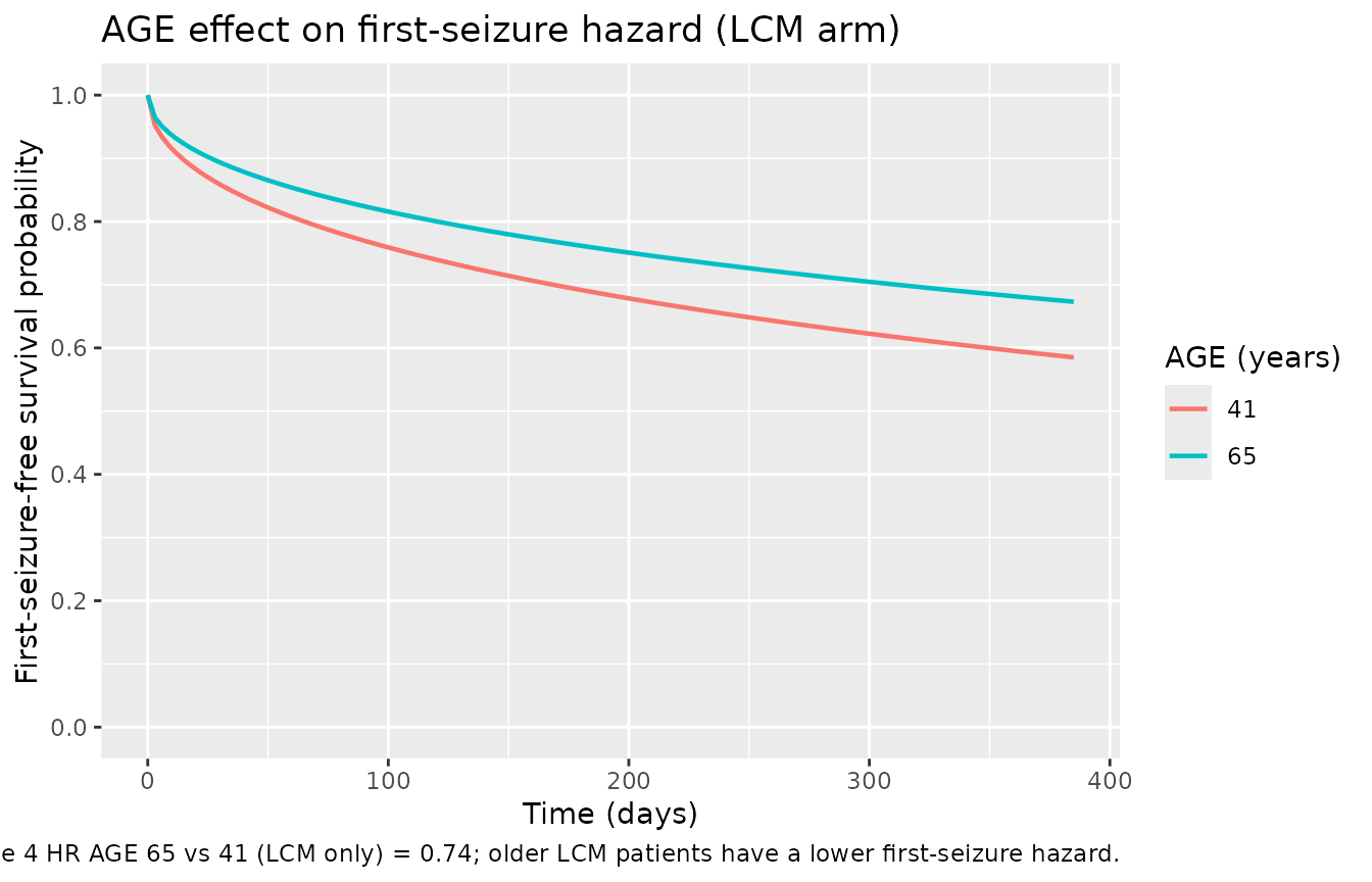
AUC dose-response check
Table 4 reports HR for LCM AUC 300 vs 100 mgh/L of 0.40 (first seizure) and 0.34 (subsequent seizures). We reproduce this contrast by simulating two LCM cohorts at daily AUC 100 mgh/L (dose level 1) and 300 mgh/L (dose level 3; LCM 600 mg/day gives approximately AUC = 312 mgh/L per the paper’s scaling).
auc_events <- tibble::tibble(
  id = 1:2, AGE = 41L, SEXF = 0L,
  CONMED_LCM = 1L, NSP3M_LT2 = 0L, NSP3M_7_50 = 0L, NSP3M_GT50 = 0L,
  AUC_LCM = c(100, 300), AUC_CBZ = 0
) |>
  tidyr::crossing(time = obs_times) |>
  dplyr::mutate(evid = 0L, amt = 0)

sim_auc <- rxode2::rxSolve(mod_seiz_typical, events = auc_events,
                           keep = c("AUC_LCM"))
#> ℹ omega/sigma items treated as zero: 'etallam_2nd'
#> Warning: multi-subject simulation without without 'omega'
sim_auc |>
  dplyr::group_by(time, AUC_LCM) |>
  dplyr::summarise(sur = mean(sur), sur_2nd = mean(sur_2nd), .groups = "drop") |>
  tidyr::pivot_longer(c(sur, sur_2nd), names_to = "hazard", values_to = "S") |>
  dplyr::mutate(hazard = dplyr::recode(hazard,
                                       sur     = "first seizure",
                                       sur_2nd = "subsequent seizure")) |>
  ggplot(aes(time, S, colour = factor(AUC_LCM))) +
  geom_line(linewidth = 0.8) +
  facet_wrap(~hazard) +
  scale_y_continuous(limits = c(0, 1), breaks = seq(0, 1, 0.2)) +
  labs(x = "Time (days)", y = "Seizure-free survival probability",
       colour = "Daily AUC LCM (mg*h/L)",
       title = "LCM AUC dose-response on the seizure hazard",
       caption = "Table 4 HRs vs the 100 mg*h/L reference: first seizure 0.40; subsequent 0.34.")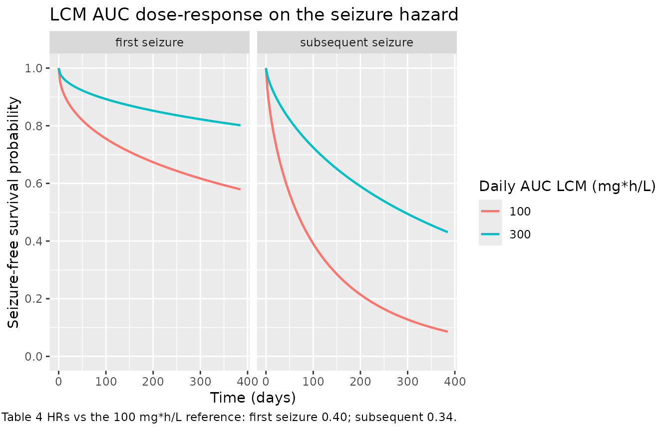
NCA validation
Not applicable. The Lindauer 2017 model is a time-to-event / dropout
hazard model, not a plasma-concentration popPK model. Drug exposure
enters both sub-models as a per-subject daily AUC covariate
(AUC_LCM or AUC_CBZ) that the paper computes
from an upstream popPK model (Section 2.3) and treats as a data column;
the model file therefore has no dosing compartment and no
plasma-concentration output. Standard validation for TTE models is the
Kaplan-Meier VPC and hazard-ratio spot check shown above.
Assumptions and deviations
-
Upstream popPK models are not part of this
extraction. Lindauer 2017 Section 2.3 refers to “a previously
published population pharmacokinetic model for CBZ-CR” and “a previously
developed population pharmacokinetic model for LCM” that produced the
per-subject daily AUC used as the exposure covariate. Neither upstream
model was available when these models were built; the model files
therefore expose
AUC_LCMandAUC_CBZas data covariates and leave it to downstream users to supply per-subject AUC values (either from an external popPK simulation or from a fixed daily-dose scaling). The typical dose-to-AUC scaling used in the vignette (LCM 200 mg/day -> ~104 mgh/L; LCM 400 mg/day -> ~208 mgh/L; LCM 600 mg/day -> ~312 mgh/L; CBZ-CR 400 mg/day -> ~132 mgh/L) is the paper’s typical-value scaling stated in Table 3 note- and Section 3.4.
-
AGE effect gating by treatment arm. Table 3 lists
AGE * k1as applicable to LCM only; the model file gates the effect insidemodel()viae_age_1st * CONMED_LCM * (AGE - 41). This preserves the treatment-age interaction from the paper. -
NSP3M categorisation. The source paper’s NSP3M
variable is a raw seizure-count covariate that the authors split into
four categories (<2, 2-6, 7-50, >50) with 2-6 as reference. Per
the standing maintainer policy (“count covariate -> decomposed binary
indicators”) the extraction encodes three binary indicators
NSP3M_LT2,NSP3M_7_50,NSP3M_GT50(all zero selects the reference). Data assemblers must enforce mutual exclusivity: at most one of the three is 1 per subject. -
CONMED_LCM as a treatment-arm indicator. In the
SP0993 parallel-group monotherapy trial the covariate flags arm
membership rather than a concomitant medication. The canonical
CONMED_<INN>family is used because a patient on the LCM arm is by definition taking lacosamide; in trials with cross-over or on-off transitions the same indicator would be time-varying. - No IIV on the dropout model. Lindauer 2017 Table 2 does not report an IIV row for the dropout hazard. No eta parameters are added; the dropout simulations are therefore typical-value trajectories.
-
Placeholder additive residual on
sur. Both model files attach a small additive residual (addSd = 0.001) to the primary survivor-function output so the nlmixr2 likelihood machinery accepts the model in a fit-ready form. This is a translation artefact, not from the source. Forward simulation does not use this residual (zeroRe()in this vignette zeroes it out). -
Repeated-time-to-event two-sub-model structure. The
paper uses a NONMEM
SCOUNTcounter to switch between the first-seizure and 2nd+ seizure hazards within a single hazard-integration state during fitting. In this rxode2 forward-simulation translation we expose the two hazards as separate compartments (cumhaz_1standcumhaz_2nd) with distinct Weibull scale / shape and distinct covariate effects, so the vignette can plot the two sub-model survivor functions independently. The paper’s simulation-time gating (post-seizure the patient transitions from the 1st- to the 2nd+-sub-model) would require an external simulation loop that resets the compartment ODE origin after each simulated seizure; that logic is not built into the model file.