Model and source
- Citation: Zou J, Chen S, Rao W, Fu L, Zhang J, Liao Y, Zhang Y, Lv N, Deng G, Yang S, Lin L, Li L, Liu S, Qu J. Population pharmacokinetic modeling of bedaquiline among multidrug-resistant pulmonary tuberculosis patients from China. Antimicrob Agents Chemother. 2022;66(10):e00811-22. doi:10.1128/aac.00811-22.
- Description: One-compartment population PK model with first-order absorption for oral bedaquiline in 99 Chinese patients with multidrug-resistant pulmonary tuberculosis sampled during the 200 mg three-times-weekly continuation phase (Zou 2022). Apparent clearance decreases with serum gamma-glutamyl transferase (GGT) as a power function centred on the dataset median of 28.9 U/L, and is lowered by an additive 1.4 L/h in patients homozygous GG at AGBL4 rs319952 (reference AA + AG). Typical values CL/F = 4.54 L/h, Vc/F = 227 L, Ka = 0.447 1/h; exponential IIV on CL/F and Vc/F and a proportional residual error.
- Article: https://doi.org/10.1128/aac.00811-22 (open access, PMC9578397)
Zou 2022 developed a population PK model for oral bedaquiline (BDQ) from 246 plasma concentrations in 99 Chinese adults with multidrug-resistant pulmonary tuberculosis, sampled during the 200 mg three-times-weekly continuation phase. A one-compartment model with first-order absorption described the data. Two covariates were retained on apparent clearance (CL/F): serum gamma-glutamyl transferase (GGT) as a power term centred on the dataset median (28.9 U/L), and the AGBL4 rs319952 GG genotype as an additive shift. The final covariate model (Results Equations 1 and 2) is
The genotype effect is an absolute 1.4 L/h reduction, not a fractional one; this is the one point where reproducing the published simulation table pins the structural form unambiguously (see below).
Population
str(readModelDb("Zou_2022_bedaquiline")()$population)
#> List of 15
#>  $ species       : chr "human"
#>  $ n_subjects    : int 99
#>  $ n_studies     : int 1
#>  $ n_observations: chr "246 plasma bedaquiline concentrations (1-8 per patient; 38 patients contributed a single sample). One sample be"| __truncated__
#>  $ age_range     : chr "11-78 years"
#>  $ age_mean      : chr "38.1 years (SD 14.1)"
#>  $ weight_range  : chr "17-90.7 kg"
#>  $ weight_mean   : chr "58 kg (SD 12.6)"
#>  $ height_mean   : chr "166.4 cm (SD 12.4)"
#>  $ sex_female_pct: num NA
#>  $ race_ethnicity: Named num 100
#>   ..- attr(*, "names")= chr "Asian"
#>  $ disease_state : chr "Multidrug-resistant pulmonary tuberculosis."
#>  $ dose_range    : chr "Approved regimen: 400 mg orally once daily for 2 weeks, then 200 mg three times per week for 22 weeks. Samples "| __truncated__
#>  $ regions       : chr "China (single centre, Shenzhen Third People's Hospital)."
#>  $ notes         : chr "Recruited October 2020 to October 2021. GGT mean 36.4 U/L (range 8-271.8); ALB mean 46.2 g/L (Table 1). AGBL4 r"| __truncated__
The analysis cohort was 99 patients (mean age 38.1 years, range 11-78; mean weight 58 kg, range 17-90.7) recruited October 2020 to October 2021 at a single centre in Shenzhen. GGT averaged 36.4 U/L (range 8-271.8). AGBL4 rs319952 genotypes were AA/AG/GG = 31/39/13, with 16 of 99 ungenotyped and imputed to the most frequent class (AG). The sex split of the cohort is not reported, so it is not simulated here.
Source trace
Every value is also traced in a comment beside its ini()
line in
inst/modeldb/specificDrugs/Zou_2022_bedaquiline.R.
| Quantity | Value | Source |
|---|---|---|
| Ka | 0.447 1/h | Table 3, Ka row |
| CL/F (typical, GGT = 28.9, AA/AG) | 4.54 L/h | Table 3, CL/F row; Results Eq. 1 |
| Vc/F | 227 L | Table 3, Vc/F row |
| GGT power exponent on CL/F | -0.476 | Table 3, “u GGT on CL/F”; Results Eq. 1 |
| rs319952 GG additive shift on CL/F | -1.4 L/h | Table 3, “u rs319952 on CL/F”; Results Eq. 2 |
| GGT centring value | 28.9 U/L | Results Eqs. 1-2 (dataset median) |
| IIV CL/F | 38.7% | Table 3, h(CL/F) |
| IIV Vc/F | 83.5% | Table 3, h(Vc/F) |
| Proportional residual | 32.2% | Table 3, eps prop |
The IIV percentages are read as coefficients of variation, so the
internal variance is log(1 + CV^2); the table does not
state the convention, but the distinction is immaterial for the
deterministic replication of Table 4 below (which uses typical values
only).
Reproducing the published dosage simulation (Table 4)
Zou 2022 Table 4 reports the steady-state weekly AUC, Cmax, and Cmin for eight typical-patient scenarios: two rs319952 strata x four GGT levels (10, 30, 50, 100 U/L), under 200 mg three times weekly. We reproduce it with the typical (zero-eta) model. The three weekly doses are evenly spaced (every 56 h), which is what matches the published numbers.
modTyp <- rxode2::zeroRe(rxode2::rxode(readModelDb("Zou_2022_bedaquiline")))
#> ℹ parameter labels from comments will be replaced by 'label()'

# 200 mg TIW, doses every 56 h, 30 weeks to steady state.
doseTimes <- sort(as.vector(outer(c(0, 56, 112), 168 * (0:29), "+")))

grid <- expand.grid(
  GGT = c(10, 30, 50, 100),
  GG = c(0L, 1L)
)

simOne <- function(GGT, GG) {
  ev <- rxode2::et(amt = 200, time = doseTimes, cmt = "depot")
  ev <- rxode2::et(ev, seq(168 * 29, 168 * 30, by = 0.1), cmt = "central")
  d <- as.data.frame(ev)
  d$GGT <- GGT
  d$SNP_AGBL4_RS319952_GG <- GG
  r <- rxode2::rxSolve(modTyp, d, returnType = "data.frame")
  r <- r[r$time >= 168 * 29, ]
  data.frame(
    genotype = ifelse(GG == 1L, "G", "A&AG"),
    GGT = GGT,
    aucweekly = sum(diff(r$time) * (head(r$Cc, -1) + tail(r$Cc, -1)) / 2),
    cmax = max(r$Cc),
    cmin = min(r$Cc)
  )
}

simTab <- do.call(rbind, Map(simOne, grid$GGT, grid$GG))
#> ℹ omega/sigma items treated as zero: 'etalcl', 'etalvc'
#> ℹ omega/sigma items treated as zero: 'etalcl', 'etalvc'
#> ℹ omega/sigma items treated as zero: 'etalcl', 'etalvc'
#> ℹ omega/sigma items treated as zero: 'etalcl', 'etalvc'
#> ℹ omega/sigma items treated as zero: 'etalcl', 'etalvc'
#> ℹ omega/sigma items treated as zero: 'etalcl', 'etalvc'
#> ℹ omega/sigma items treated as zero: 'etalcl', 'etalvc'
#> ℹ omega/sigma items treated as zero: 'etalcl', 'etalvc'

published <- tibble::tribble(
  ~genotype, ~GGT, ~aucweekly_pub, ~cmax_pub, ~cmin_pub,
  "A&AG", 10, 79.746, 0.859, 0.176,
  "A&AG", 30, 134.529, 1.165, 0.460,
  "A&AG", 50, 171.561, 1.377, 0.666,
  "A&AG", 100, 238.620, 1.767, 1.051,
  "G", 10, 97.977, 0.959, 0.266,
  "G", 30, 196.080, 1.519, 0.806,
  "G", 50, 286.080, 2.046, 1.328,
  "G", 100, 538.383, 3.538, 2.815
)

cmp <- simTab |>
  dplyr::left_join(published, by = c("genotype", "GGT")) |>
  dplyr::mutate(
    AUCweekly = sprintf("%.1f / %.1f", aucweekly, aucweekly_pub),
    Cmax = sprintf("%.3f / %.3f", cmax, cmax_pub),
    Cmin = sprintf("%.3f / %.3f", cmin, cmin_pub)
  ) |>
  dplyr::select(genotype, GGT, AUCweekly, Cmax, Cmin) |>
  dplyr::rename(
    "rs319952" = genotype,
    "GGT (U/L)" = GGT,
    "AUCweekly (sim / pub)" = AUCweekly,
    "Cmax (sim / pub)" = Cmax,
    "Cmin (sim / pub)" = Cmin
  )

knitr::kable(
  cmp,
  caption = "Simulated vs. Zou 2022 Table 4 (mg/L and mg/L*h).",
  align = c("l", "r", "r", "r", "r")
)| rs319952 | GGT (U/L) | AUCweekly (sim / pub) | Cmax (sim / pub) | Cmin (sim / pub) |
|---|---|---|---|---|
| A&AG | 10 | 79.7 / 79.7 | 0.859 / 0.859 | 0.176 / 0.176 |
| A&AG | 30 | 134.5 / 134.5 | 1.165 / 1.165 | 0.460 / 0.460 |
| A&AG | 50 | 171.6 / 171.6 | 1.378 / 1.377 | 0.666 / 0.666 |
| A&AG | 100 | 238.6 / 238.6 | 1.770 / 1.767 | 1.051 / 1.051 |
| G | 10 | 98.0 / 98.0 | 0.959 / 0.959 | 0.266 / 0.266 |
| G | 30 | 196.1 / 196.1 | 1.521 / 1.519 | 0.806 / 0.806 |
| G | 50 | 286.1 / 286.1 | 2.049 / 2.046 | 1.328 / 1.328 |
| G | 100 | 538.4 / 538.4 | 3.542 / 3.538 | 2.815 / 2.815 |
# Hard gate: the replication reproduces the published table to within rounding.
stopifnot(
  max(abs(simTab$aucweekly - published$aucweekly_pub)) < 0.5,
  max(abs(simTab$cmax - published$cmax_pub)) < 0.01,
  max(abs(simTab$cmin - published$cmin_pub)) < 0.01
)
Every cell agrees with the paper to three significant figures.
Because the weekly AUC is exactly 600 / (CL/F) (three 200
mg doses per week divided by the apparent clearance), the AUC column
alone would already pin CL/F; the GG-stratum AUCs only reconcile when
the 1.4 L/h genotype effect is applied additively after
the GGT power term, confirming the structural form.
Steady-state concentration-time profiles (Figure 3)
profile <- function(GGT, GG) {
  ev <- rxode2::et(amt = 200, time = doseTimes, cmt = "depot")
  ev <- rxode2::et(ev, seq(168 * 29, 168 * 30, by = 0.25), cmt = "central")
  d <- as.data.frame(ev)
  d$GGT <- GGT
  d$SNP_AGBL4_RS319952_GG <- GG
  r <- rxode2::rxSolve(modTyp, d, returnType = "data.frame")
  r <- r[r$time >= 168 * 29, ]
  data.frame(
    time = r$time - 168 * 29,
    Cc = r$Cc,
    GGT = factor(GGT),
    genotype = ifelse(GG == 1L, "rs319952 GG", "rs319952 AA & AG")
  )
}

prof <- do.call(rbind, Map(profile, grid$GGT, grid$GG))
#> ℹ omega/sigma items treated as zero: 'etalcl', 'etalvc'
#> ℹ omega/sigma items treated as zero: 'etalcl', 'etalvc'
#> ℹ omega/sigma items treated as zero: 'etalcl', 'etalvc'
#> ℹ omega/sigma items treated as zero: 'etalcl', 'etalvc'
#> ℹ omega/sigma items treated as zero: 'etalcl', 'etalvc'
#> ℹ omega/sigma items treated as zero: 'etalcl', 'etalvc'
#> ℹ omega/sigma items treated as zero: 'etalcl', 'etalvc'
#> ℹ omega/sigma items treated as zero: 'etalcl', 'etalvc'

ggplot(prof, aes(time, Cc, colour = GGT)) +
  geom_line() +
  facet_wrap(~genotype) +
  labs(
    x = "Time within a steady-state week (h)",
    y = "Bedaquiline (mg/L)",
    colour = "GGT (U/L)",
    title = "Replicates Figure 3 of Zou 2022"
  ) +
  theme_bw()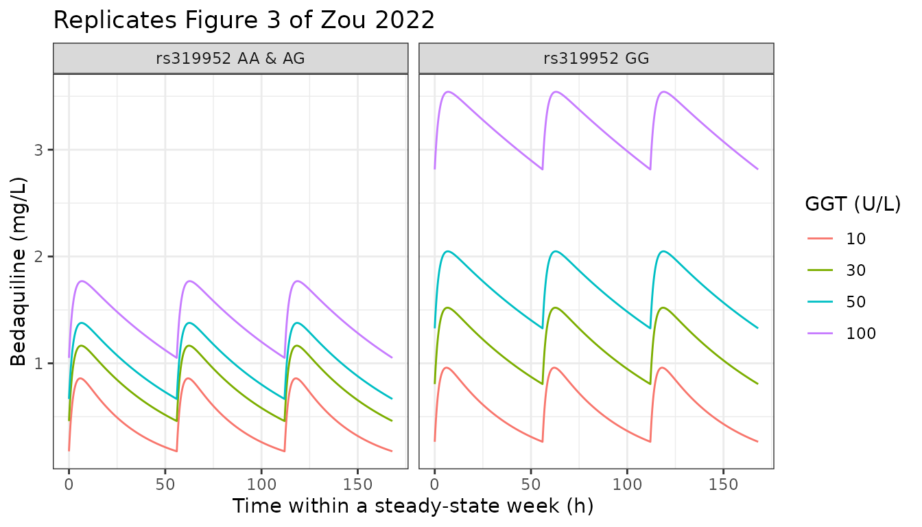
PKNCA validation
We confirm the steady-state exposures with PKNCA for the reference scenario (GGT = 30 U/L, each genotype), computing over one 168 h steady-state week.
ncaScenarios <- expand.grid(GGT = 30, GG = c(0L, 1L))

concList <- Map(function(GGT, GG) {
  ev <- rxode2::et(amt = 200, time = doseTimes, cmt = "depot")
  ev <- rxode2::et(ev, seq(168 * 29, 168 * 30, by = 0.1), cmt = "central")
  d <- as.data.frame(ev)
  d$GGT <- GGT
  d$SNP_AGBL4_RS319952_GG <- GG
  r <- rxode2::rxSolve(modTyp, d, returnType = "data.frame")
  r <- r[r$time >= 168 * 29, ]
  data.frame(
    id = 1L,
    treatment = ifelse(GG == 1L, "G", "A&AG"),
    time = r$time - 168 * 29,
    Cc = r$Cc
  )
}, ncaScenarios$GGT, ncaScenarios$GG)
#> ℹ omega/sigma items treated as zero: 'etalcl', 'etalvc'
#> ℹ omega/sigma items treated as zero: 'etalcl', 'etalvc'

conc <- dplyr::bind_rows(concList) |>
  dplyr::filter(!is.na(Cc))

dose <- conc |>
  dplyr::group_by(treatment) |>
  dplyr::summarise(time = 0, amt = 200, .groups = "drop") |>
  dplyr::mutate(id = 1L)

ncaData <- PKNCA::PKNCAdata(
  PKNCA::PKNCAconc(conc, Cc ~ time | treatment),
  PKNCA::PKNCAdose(dose, amt ~ time | treatment),
  intervals = data.frame(
    start = 0, end = 168,
    cmax = TRUE, cmin = TRUE, auclast = TRUE
  )
)
ncaRes <- PKNCA::pk.nca(ncaData)

ncaWide <- as.data.frame(ncaRes) |>
  dplyr::select(treatment, PPTESTCD, PPORRES) |>
  tidyr::pivot_wider(names_from = PPTESTCD, values_from = PPORRES)

knitr::kable(
  ncaWide |>
    dplyr::rename(
      "rs319952" = treatment,
      "Cmax (mg/L)" = cmax,
      "Cmin (mg/L)" = cmin,
      "AUC0-168h (mg/L*h)" = auclast
    ),
  digits = 3,
  caption = "PKNCA steady-state NCA over one 168 h week at GGT = 30 U/L."
)| rs319952 | AUC0-168h (mg/L*h) | Cmax (mg/L) | Cmin (mg/L) |
|---|---|---|---|
| A&AG | 134.529 | 1.165 | 0.460 |
| G | 196.078 | 1.521 | 0.806 |
# The PKNCA weekly AUC must match the published Table 4 AUCweekly values
# (134.5 for A&AG, 196.1 for G at GGT = 30).
aucByTrt <- ncaWide$auclast[match(c("A&AG", "G"), ncaWide$treatment)]
stopifnot(
  abs(aucByTrt[1] - 134.529) < 1,
  abs(aucByTrt[2] - 196.080) < 1
)
The PKNCA weekly AUC reproduces the published Table 4 values (134.5 and 196.1 mg/L*h at GGT = 30 U/L) within rounding, independently confirming the clearance parameterisation.
Assumptions and deviations
- rs319952 genotype effect is additive, not fractional. Results Equation 2 subtracts 1.4 L/h from CL/F for GG subjects. The exact reproduction of Table 4 confirms this reading; a multiplicative interpretation would miss the GG-stratum exposures badly.
- GGT centring value. The power term is centred on 28.9 U/L, the dataset median printed in Equations 1 and 2. The cohort mean (36.4 U/L) is not used.
- Dosing schedule. The paper’s Table 4 simulation uses 200 mg three times weekly; the published Cmax/Cmin only reproduce when the three weekly doses are evenly spaced (every 56 h). The clinical regimen (Monday/Wednesday/Friday) is not evenly spaced, but the authors’ simulation used even spacing, so the maintainers use it here to match the reference table.
- Sex not simulated. The cohort sex split is not reported; sex was screened on CL/F but not retained, so it does not enter the model.
- Ungenotyped subjects. 16 of 99 patients were not genotyped at rs319952 and were imputed to AG by the authors, entering the fit with the GG indicator = 0.
-
IIV convention. The Table 3 IIV percentages are
read as CVs (
omega^2 = log(1 + CV^2)); the deterministic replications above are unaffected by the choice. - No correction or erratum notice was found for this article as of 2026-10-09.