S(-)-carvedilol (Othman 2007)
Source:vignettes/articles/Othman_2007_carvedilol.Rmd
Othman_2007_carvedilol.RmdModel and source
- Citation: Othman AA, Tenero DM, Boyle DA, Eddington ND, Fossler MJ. Population pharmacokinetics of S(-)-carvedilol in healthy volunteers after administration of the immediate-release (IR) and the new controlled-release (CR) dosage forms of the racemate. AAPS J. 2007;9(2):E208-E218.
- Article: https://doi.org/10.1208/aapsj0902023
- Corrigendum (corrected alignment of Tables 1, 3, 4; numeric values unchanged): https://doi.org/10.1208/aapsj0903037c
Population
The analysis pooled 3,328 S(-)-carvedilol plasma concentrations from 96 healthy volunteers across three studies. The IR data (1,270 concentrations, 56 subjects) came from two open-label studies in which subjects took 25 mg of immediate-release carvedilol (racemate, free base) every 12 hours for two doses. The CR data (2,058 concentrations, 40 subjects) came from a nonrandomized, open-label, single-dose, dose-rising, 4-period balanced crossover study in which each subject received single doses of 10, 20, 40, and 80 mg of carvedilol phosphate (equivalent to 8.1, 16.2, 32.4, and 64.8 mg of carvedilol racemate free base) with at least one week of washout between doses. Poor metabolizers of carvedilol were excluded by CYP2D6 genotyping. All doses were administered under fed conditions (moderate-calorie, low-to-moderate-fat breakfast 30 minutes pre-dose). Demographic baseline ranges (age, weight, sex distribution) are not reported in the publication; the paper text states only that the volunteers were healthy. The analysis modelled the concentrations of the S(-) enantiomer of carvedilol (the beta-blocking enantiomer); doses were scaled to the administered S(-) free-base amount (half the racemate dose) inside the NONMEM data set.
The structured population metadata is available
programmatically:
m <- nlmixr2est::nlmixr(readModelDb("Othman_2007_carvedilol"))
#> ℹ parameter labels from comments will be replaced by 'label()'
str(m$meta$population)
#> List of 14
#>  $ species       : chr "human"
#>  $ n_subjects    : int 96
#>  $ n_studies     : int 3
#>  $ age_range     : chr "Healthy adults (specific demographic ranges not reported in the paper)"
#>  $ weight_range  : chr "Healthy adults (specific demographic ranges not reported in the paper)"
#>  $ sex_female_pct: NULL
#>  $ race_ethnicity: chr "Not reported in the paper"
#>  $ disease_state : chr "Healthy volunteers"
#>  $ dose_range    : chr "IR: 25 mg of carvedilol (racemate, free base) every 12 hours for 2 doses; CR: single doses of 10, 20, 40, or 80"| __truncated__
#>  $ regions       : chr "Not reported"
#>  $ n_observations: int 3328
#>  $ n_obs_ir      : int 1270
#>  $ n_obs_cr      : int 2058
#>  $ notes         : chr "Three pooled studies (2 IR, 1 CR). Poor metabolizers of carvedilol were excluded by CYP2D6 genotyping. All dose"| __truncated__
Source trace
The per-parameter origin is recorded as an in-file trailing comment
next to each ini() entry in
inst/modeldb/specificDrugs/Othman_2007_carvedilol.R. The
table below collects them in one place for review.
| Equation / parameter | Value | Source location |
|---|---|---|
lcl = log(CL/F) |
149 L/h | Table 1, CL/F (4.8% RSE) |
lvc = log(Vc/F) |
828 L | Table 1, Vc/F (6.6% RSE) |
lvp = log(Vp/F) |
1150 L | Table 1, Vp/F (10.3% RSE) |
lq = log(Q/F) |
94.7 L/h | Table 1, Q/F (5.3% RSE) |
lka_cr_0to2 |
0.08 1/h | Table 1, KA CR 0-2 h (16.0% RSE) |
lka_cr_2to4 |
0.27 1/h | Table 1, KA CR 2-4 h (16.1% RSE) |
lka_cr_gt4 |
3.5 1/h | Table 1, KA CR > 4 h (17.7% RSE) |
lka_iram_0to1 |
0.92 1/h | Table 1, KA IR AM 0-1 h (21.5% RSE) |
lka_iram_gt1 |
8.79 1/h | Table 1, KA IR AM > 1 h (42.1% RSE) |
lka_irpm_0to1 |
0.42 1/h | Table 1, KA IR PM 0-1 h (26.7% RSE) |
lka_irpm_gt1 |
3.0 1/h | Table 1, KA IR PM > 1 h (31.9% RSE) |
lfrel_cr |
0.76 | Table 1, Frel CR (7.4% RSE) |
lfrel_irpm |
0.80 | Table 1, Frel IR PM (3.2% RSE) |
| Frel IR AM (reference, fixed at 1) | 1 (fixed) | Table 1 footnote |
ltlag_cr |
0.23 h (fixed) | Table 1, Tlag CR (Fixed, sensitivity analysis) |
ltlag_ir |
0.20 h | Table 1, Tlag IR (5.3% RSE) |
eta var Vc/F (etalvc) |
0.14 | Table 3 final point estimate |
eta var KA CR (etalka_cr) |
0.90 | Table 3 final point estimate (one variance, three CR stages) |
eta var KA IRAM (etalka_iram) |
1.97 | Table 3 final point estimate (one variance, two IRAM stages) |
eta var KA IRPM (etalka_irpm) |
3.73 | Table 3 final point estimate (one variance, two IRPM stages) |
eta var Frel (etafrel) |
0.11 | Table 3 final point estimate (one variance shared across CR/IRAM/IRPM) |
IOV var KA CR (etalka_cr_iov) |
1.29 | Table 3 pi^2 KA,CR; per-occasion IOV (CR crossover) |
IOV var Frel CR (etafrel_cr_iov) |
0.02 | Table 3 pi^2 Frel,CR; per-occasion IOV (CR crossover) |
Residual var sigma^2 (expSd = sqrt(sigma^2)) |
0.10 | Table 3 sigma^2 = 0.10; lognormal residual error (Eq. 3) |
| Structural ODE: 2-compartment with 3 parallel depots | n/a | Methods page E209 (paragraph starting “A 2-compartment structural model parameterized in terms of clearance …”) |
| Time-varying KA via tad() switches at 2 h / 4 h (CR) and 1 h (IR) | n/a | Methods page E210 and Results page E212 (paragraph starting “the results of the sensitivity analyses indicated that 2 break points for KACR at 2 and 4 hours …”) |
| Frel IRAM as reference (= 1, fixed) | n/a | Methods page E209-E210 (“Frel was set to 1 for the IRAM dose (as the reference) …”) |
Virtual cohort
The original observed data are not publicly available. The figures below build virtual cohorts that match each dose group in the Othman 2007 design exactly: the IR design simulates a single subject taking 25 mg of carvedilol IR (racemate) every 12 hours for two doses, and the CR design simulates each of the four CR dose levels (10, 20, 40, 80 mg of carvedilol phosphate) as a separate single-dose period. Each “subject” represents a typical-value trajectory; the published Cmax / AUC summaries are taken from Table 4.
# S(-)-carvedilol mg per administered dose:
#   * IR carvedilol racemate 25 mg -> 12.5 mg S(-)-carvedilol (50/50 racemate).
#   * CR carvedilol phosphate 10 / 20 / 40 / 80 mg
#       -> carvedilol racemate free base 8.1 / 16.2 / 32.4 / 64.8 mg
#       -> S(-)-carvedilol             4.05 / 8.10 / 16.20 / 32.40 mg
#     (the 8.1/10 = 0.81 phosphate-to-free-base factor and the 0.5
#     racemate-to-enantiomer factor come from the paper's Methods section.)
ir_s_dose <- 25 * 0.5      # mg S(-)-carvedilol per IR dose (25 mg racemate)
cr_phos_doses <- c(10, 20, 40, 80)
cr_s_doses <- cr_phos_doses * 0.81 * 0.5
data.frame(
  cr_phosphate_mg = cr_phos_doses,
  cr_free_base_racemate_mg = cr_phos_doses * 0.81,
  cr_S_carvedilol_mg = cr_s_doses
)
#>   cr_phosphate_mg cr_free_base_racemate_mg cr_S_carvedilol_mg
#> 1              10                      8.1               4.05
#> 2              20                     16.2               8.10
#> 3              40                     32.4              16.20
#> 4              80                     64.8              32.40
# Build per-cohort event tables; each cohort is a typical-value simulation
# (one subject per cohort). The IR cohort takes 25 mg AM + 25 mg PM; the CR
# cohorts each take a single dose.
sample_grid <- function(times) rxode2::et(times)

ir_events <- rxode2::et(amt = ir_s_dose, cmt = "depot2", time = 0) |>
  rxode2::et(amt = ir_s_dose, cmt = "depot3", time = 12) |>
  rxode2::et(seq(0, 48, by = 0.25))

cr_event_list <- lapply(seq_along(cr_phos_doses), function(k) {
  rxode2::et(amt = cr_s_doses[k], cmt = "depot", time = 0) |>
    rxode2::et(seq(0, 48, by = 0.25))
})
names(cr_event_list) <- paste0("CR_", cr_phos_doses, "mg")
Simulation
m <- nlmixr2est::nlmixr(readModelDb("Othman_2007_carvedilol"))
#> ℹ parameter labels from comments will be replaced by 'label()'
m_typ <- rxode2::zeroRe(m)

sim_ir <- as.data.frame(rxode2::rxSolve(m_typ, ir_events)) |>
  dplyr::mutate(treatment = "IR 25 mg AM + 25 mg PM (racemate)")
#> ℹ omega/sigma items treated as zero: 'etalvc', 'etalka_cr', 'etalka_iram', 'etalka_irpm', 'etafrel', 'etalka_cr_iov', 'etafrel_cr_iov'

sim_cr <- dplyr::bind_rows(lapply(names(cr_event_list), function(label) {
  s <- as.data.frame(rxode2::rxSolve(m_typ, cr_event_list[[label]]))
  s$treatment <- label
  s
}))
#> ℹ omega/sigma items treated as zero: 'etalvc', 'etalka_cr', 'etalka_iram', 'etalka_irpm', 'etafrel', 'etalka_cr_iov', 'etafrel_cr_iov'
#> ℹ omega/sigma items treated as zero: 'etalvc', 'etalka_cr', 'etalka_iram', 'etalka_irpm', 'etafrel', 'etalka_cr_iov', 'etafrel_cr_iov'
#> ℹ omega/sigma items treated as zero: 'etalvc', 'etalka_cr', 'etalka_iram', 'etalka_irpm', 'etafrel', 'etalka_cr_iov', 'etafrel_cr_iov'
#> ℹ omega/sigma items treated as zero: 'etalvc', 'etalka_cr', 'etalka_iram', 'etalka_irpm', 'etafrel', 'etalka_cr_iov', 'etafrel_cr_iov'
Replicate published figures
Figure 1 – representative IR (25 mg AM + 25 mg PM) and CR profiles
# Replicates the IR panel (Figure 1A) of Othman 2007: representative IR
# 25 mg q12h concentration-time profile in healthy volunteers.
ggplot(sim_ir, aes(time, Cc)) +
  geom_line() +
  labs(x = "Time (h)", y = "S(-)-carvedilol concentration (ng/mL)",
       title = "Typical IR carvedilol 25 mg q12h profile",
       caption = "Reproduces Figure 1A of Othman 2007 (typical-value simulation).")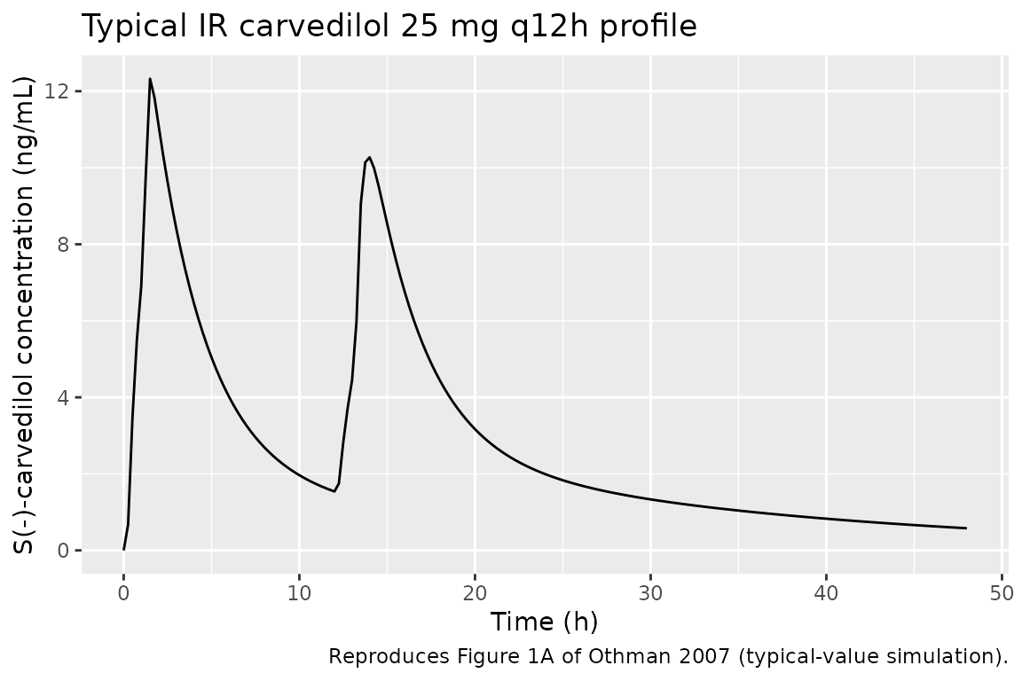
# Replicates the CR panel (Figure 1B) of Othman 2007: representative CR
# concentration-time profile at the 20 mg dose level (one of the four
# CR doses in the crossover).
ggplot(dplyr::filter(sim_cr, treatment == "CR_20mg"),
       aes(time, Cc)) +
  geom_line() +
  labs(x = "Time (h)", y = "S(-)-carvedilol concentration (ng/mL)",
       title = "Typical CR carvedilol 20 mg profile",
       caption = "Reproduces Figure 1B of Othman 2007 (typical-value simulation).")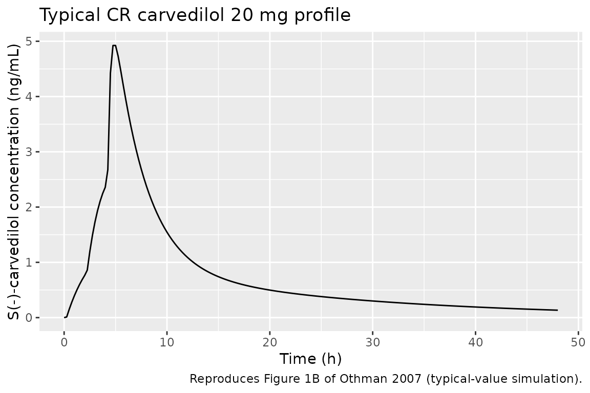
Figure 4 – CR concentration-time profiles, dose-stratified
# Replicates Figure 4 of Othman 2007: dose-stratified CR concentration-time
# profiles (10/20/40/80 mg phosphate).
ggplot(sim_cr, aes(time, Cc, colour = treatment)) +
  geom_line() +
  labs(x = "Time (h)", y = "S(-)-carvedilol concentration (ng/mL)",
       colour = "Treatment",
       title = "Typical CR carvedilol profiles (dose-rising crossover)",
       caption = "Reproduces Figure 4 of Othman 2007 (typical-value simulation).")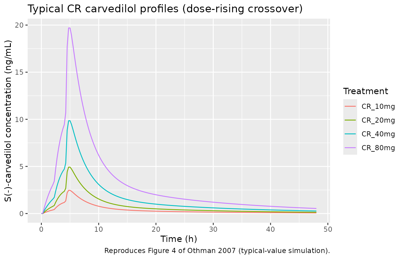
PKNCA validation
For NCA the IR AM and IR PM doses are extracted into separate per-subject NCA records so that AUC0-12 (IR AM, dose period 1) and AUC12-48 (IR PM, dose period 2) can be compared to Table 4. Each CR dose level is its own subject.
nca_subjects <- dplyr::bind_rows(
  # IR AM (period 1, 0-12 h)
  sim_ir |>
    dplyr::filter(time <= 12) |>
    dplyr::transmute(id = 1L, time = time, Cc = Cc,
                     treatment = "IR 25 mg (am)"),
  # IR PM (period 2, 12-48 h; reset time to 0 at the PM dose for NCA)
  sim_ir |>
    dplyr::filter(time >= 12) |>
    dplyr::transmute(id = 2L, time = time - 12, Cc = Cc,
                     treatment = "IR 25 mg (pm)"),
  # CR doses (each cohort is its own id)
  sim_cr |>
    dplyr::group_by(treatment) |>
    dplyr::mutate(id = match(treatment, paste0("CR_", cr_phos_doses, "mg")) + 2L) |>
    dplyr::ungroup() |>
    dplyr::transmute(id = id, time = time, Cc = Cc,
                     treatment = paste0("CR ", sub("CR_", "", treatment)))
)

nca_doses <- dplyr::bind_rows(
  data.frame(id = 1L, time = 0,  amt = ir_s_dose, treatment = "IR 25 mg (am)"),
  data.frame(id = 2L, time = 0,  amt = ir_s_dose, treatment = "IR 25 mg (pm)"),
  data.frame(id = 3L:6L, time = 0,
             amt = cr_s_doses,
             treatment = paste0("CR ", cr_phos_doses, "mg"))
)

conc_obj <- PKNCA::PKNCAconc(
  data = nca_subjects, Cc ~ time | treatment + id,
  concu = "ng/mL", timeu = "h"
)
dose_obj <- PKNCA::PKNCAdose(
  data = nca_doses, amt ~ time | treatment + id,
  doseu = "mg"
)
# Per Table 4 of Othman 2007: AUC was integrated 0-12 h (IRAM), 12-48 h (IRPM),
# and 0-48 h (CR). For PKNCA we use auclast on each per-subject window, which
# spans the simulated record above for each cohort.
intervals <- data.frame(
  start   = 0,
  end     = c(12, 36, 48, 48, 48, 48),  # IRAM, IRPM (12-48 -> 0-36), CR 10/20/40/80
  cmax    = TRUE,
  tmax    = TRUE,
  auclast = TRUE,
  treatment = c("IR 25 mg (am)", "IR 25 mg (pm)",
                "CR 10mg", "CR 20mg", "CR 40mg", "CR 80mg")
)

nca <- PKNCA::pk.nca(PKNCA::PKNCAdata(conc_obj, dose_obj, intervals = intervals))
nca_summary <- as.data.frame(nca$result)
knitr::kable(
  dplyr::select(nca_summary, treatment, start, end, PPTESTCD, PPORRES),
  caption = "Simulated NCA parameters (typical-value, no IIV)."
)| treatment | start | end | PPTESTCD | PPORRES |
|---|---|---|---|---|
| IR 25 mg (am) | 0 | 12 | auclast | 55.871654 |
| IR 25 mg (am) | 0 | 12 | cmax | 12.325160 |
| IR 25 mg (am) | 0 | 12 | tmax | 1.500000 |
| IR 25 mg (pm) | 0 | 36 | auclast | 82.209361 |
| IR 25 mg (pm) | 0 | 36 | cmax | 10.272331 |
| IR 25 mg (pm) | 0 | 36 | tmax | 2.000000 |
| CR 10mg | 0 | 48 | auclast | 19.132521 |
| CR 10mg | 0 | 48 | cmax | 2.462129 |
| CR 10mg | 0 | 48 | tmax | 5.000000 |
| CR 20mg | 0 | 48 | auclast | 38.265040 |
| CR 20mg | 0 | 48 | cmax | 4.924256 |
| CR 20mg | 0 | 48 | tmax | 5.000000 |
| CR 40mg | 0 | 48 | auclast | 76.530086 |
| CR 40mg | 0 | 48 | cmax | 9.848514 |
| CR 40mg | 0 | 48 | tmax | 5.000000 |
| CR 80mg | 0 | 48 | auclast | 153.060172 |
| CR 80mg | 0 | 48 | cmax | 19.697026 |
| CR 80mg | 0 | 48 | tmax | 5.000000 |
Comparison against published NCA (Table 4)
# Pivot the simulated NCA to a wide table by parameter.
sim_tbl <- nca_summary |>
  dplyr::select(treatment, PPTESTCD, PPORRES) |>
  tidyr::pivot_wider(names_from = PPTESTCD, values_from = PPORRES) |>
  dplyr::rename(Cmax_sim = cmax, Tmax_sim = tmax, AUC_sim = auclast)

# Othman 2007 Table 4 -- observed medians and 90% prediction intervals from
# the model. Cc units ng/mL; AUC in ng*h/mL.
published <- tibble::tribble(
  ~treatment,        ~Cmax_pub_median,  ~Cmax_pub_PI,         ~Tmax_pub_median,  ~Tmax_pub_PI,    ~AUC_pub_median,  ~AUC_pub_PI,
  "CR 10mg",         1.81,              "1.80-3.22",          6,                 "4-6",           12.75,            "11.66-21.74",
  "CR 20mg",         3.76,              "3.52-6.53",          5,                 "4.5-6",         31.77,            "27.65-48.67",
  "CR 40mg",         8.13,              "6.99-13.23",         5,                 "4.5-6",         71.29,            "57.80-98.50",
  "CR 80mg",         17.87,             "14.02-25.75",        5,                 "4.5-6",         145.59,           "116.73-193.73",
  "IR 25 mg (am)",   15.65,             "11.62-15.03",        1.5,               "1.5-2",         59.65,            "48.80-61.39",
  "IR 25 mg (pm)",   12.6,              "9.54-12.81",         14,                "13.5-14",       83.5,             "75.19-93.72"
)

comparison <- dplyr::left_join(published, sim_tbl, by = "treatment") |>
  dplyr::select(treatment,
                Cmax_sim, Cmax_pub_median, Cmax_pub_PI,
                Tmax_sim, Tmax_pub_median, Tmax_pub_PI,
                AUC_sim, AUC_pub_median, AUC_pub_PI)
knitr::kable(comparison,
             digits = 2,
caption = "Side-by-side: typical-value simulation vs Othman 2007 Table 4 (observed medians and model 90% prediction intervals). IR PM Tmax_sim is measured from the PM dose record (time 0 = PM dose), matching the paper's convention.")| treatment | Cmax_sim | Cmax_pub_median | Cmax_pub_PI | Tmax_sim | Tmax_pub_median | Tmax_pub_PI | AUC_sim | AUC_pub_median | AUC_pub_PI |
|---|---|---|---|---|---|---|---|---|---|
| CR 10mg | 2.46 | 1.81 | 1.80-3.22 | 5.0 | 6.0 | 4-6 | 19.13 | 12.75 | 11.66-21.74 |
| CR 20mg | 4.92 | 3.76 | 3.52-6.53 | 5.0 | 5.0 | 4.5-6 | 38.27 | 31.77 | 27.65-48.67 |
| CR 40mg | 9.85 | 8.13 | 6.99-13.23 | 5.0 | 5.0 | 4.5-6 | 76.53 | 71.29 | 57.80-98.50 |
| CR 80mg | 19.70 | 17.87 | 14.02-25.75 | 5.0 | 5.0 | 4.5-6 | 153.06 | 145.59 | 116.73-193.73 |
| IR 25 mg (am) | 12.33 | 15.65 | 11.62-15.03 | 1.5 | 1.5 | 1.5-2 | 55.87 | 59.65 | 48.80-61.39 |
| IR 25 mg (pm) | 10.27 | 12.60 | 9.54-12.81 | 2.0 | 14.0 | 13.5-14 | 82.21 | 83.50 | 75.19-93.72 |
Assumptions and deviations
-
Three parallel depot compartments encode the dosage
form:
depotcarries CR,depot2carries IR morning, anddepot3carries IR evening. The user picks the formulation by setting thecmtcolumn on the dose record. This matches Othman 2007’s NONMEM ADVAN-4 / TRANS-4 parameterisation, where the diurnal IR and the CR forms had independent absorption parameters. -
Time-varying KA via
tad()switches. The model usesif (tad(depot) >= 2) ...and analogous statements to switch the absorption rate constant at the published break points (2 h and 4 h for CR; 1 h for each IR direction).tad(<depot>)returns time since the most recent dose into the named compartment, so the switches fire correctly even in multi-dose simulations. -
IIV mu-referencing workaround. rxode2’s
mu-referencing parser currently rejects
exp(theta + eta1 + eta2)(a single exp call carrying two etas). The model’s IOV terms (etalka_cr_iov,etafrel_cr_iov) are therefore factored as a separateiov_<param> <- exp(eta_<param>_iov)multiplier applied to the typical-valueexp(theta + eta_<param>)expression. The mathematical result is identical (exp(theta + eta + eta_iov)=exp(theta + eta) * exp(eta_iov)). -
IOV encoded as paper-specific etas, not
per-occasion. Othman 2007’s Eq. 2 introduces kappa terms that
are re-sampled at each CR study occasion (10, 20, 40, 80 mg in the same
subject). For the model library these are encoded as additional
per-subject etas (
etalka_cr_iov,etafrel_cr_iov) declared viapaper_specific_etas. In a stochastic simulation these are sampled once per subject, which under-counts the source design’s per-occasion variability. A user who needs per-occasion IOV can post-process by re-sampling these etas at each CR dose (rxode2’siovmachinery or a custom event-table construction). -
Residual error simplification: no eta on epsilon.
Othman 2007 uses Eq. 4
(
ln Yobs = ln Ypred + epsilon * exp(eta_RES)), an additional log-normal IIV on the residual SD itself (Table 3 omega^2 RES_ERR = 0.05). This layer is omitted from the packaged model; the residual is the standard log-normalCc ~ lnorm(expSd)withexpSd = sqrt(0.10) ~ 0.3162. For typical-value simulations (used in this vignette) the eta-on-epsilon term has no effect; for stochastic VPCs it would broaden the residual distribution by a modest factor (~5% on log scale). -
No covariates retained. Othman 2007 did not include
any baseline demographic covariates in the final model: “incorporation
of intersubject variability on Cl/F, Vp/F, and Q/F did not significantly
improve the fit (P > .05), and as a result they were omitted from the
model.” The model file therefore declares
covariateData <- list(). -
CR Tlag fixed at 0.23 h. The paper notes that
estimation of TlagCR gave rounding errors in NONMEM (error code 134) and
was therefore fixed at 0.23 h based on a sensitivity analysis. The model
file wraps this in
fixed(). -
Dose conversion for simulation. The model’s dose
variable is mg of S(-)-carvedilol free base. For CR, the paper’s nominal
dose is in mg of carvedilol phosphate; convert via
S(-)-mg = phosphate_mg * 0.81 * 0.5(the 0.81 ratio comes from 8.1 mg free base per 10 mg phosphate; the 0.5 ratio is the 50:50 racemic split). For IR, the paper’s nominal dose is in mg of carvedilol racemate free base; convert viaS(-)-mg = racemate_mg * 0.5. -
Corrigendum. The on-disk source file is the AAPS J
2007 corrigendum (doi:10.1208/aapsj0903037c), which republished Tables 1,
3, and 4 with corrected column alignment. The numeric values are
unchanged between the original publication and the corrigendum; the
corrigendum citation appears in the model’s
referencefield. The original Othman 2007 (AAPS J 9(2):E208-E218; PMC2751410) was obtained from Europe PMC for the Methods, Results narrative, and Tables 2 / Figures 1-5 (not republished in the corrigendum). -
Population demographics not reported. The
publication does not give the numeric ranges for age, weight, sex, or
race of the 96 volunteers; the Methods section states only that they
were healthy adult CYP2D6 non-poor metabolizers. The
populationmetadata therefore carries placeholder strings for these fields, and the virtual cohort below is a typical-value simulation (a single representative subject per dose group) rather than a demographic-distribution-based stochastic VPC.