Quinidine BBB transport in kainate-treated rats (Syvanen 2012)
Source:vignettes/articles/Syvanen_2012_quinidine_rat.Rmd
Syvanen_2012_quinidine_rat.RmdModel and source
- Citation: Syvanen S, Schenke M, van den Berg D-J, Voskuyl RA, de Lange ECM. Alteration in P-glycoprotein Functionality Affects Intrabrain Distribution of Quinidine More Than Brain Entry – A Study in Rats Subjected to Status Epilepticus by Kainate. AAPS J. 2012;14(1):87-96. doi:[10.1208/s12248-011-9318-1](https://doi.org/10.1208/s12248-011-9318-1).
The packaged model is a faithful translation of the paper’s final NONMEM VI ADVAN6 fit (paper Figure 2 schematic, Table II “Estimation” column, Table IV equations). It is a preclinical (rat) brain-microdialysis popPK model with:
- Two-compartment plasma disposition (central plasma
V1, peripheral plasmaV2, inter-compartmental clearanceQ, systemic clearanceCL). - A brain extracellular fluid (ECF) compartment
V_Brsampled by hippocampal microdialysis, exchanging with central plasma via asymmetric BBB clearances (Q_infor influx,Q_outfor efflux). The paper parameterisesQ_in = f1 * Q_outwithQ_outFIXED at 10.8 mL/min from a bootstrap-stability analysis. - A third observed output, total brain tissue concentration
C_brain_deep, modelled as the algebraic equilibrium multipleC_brain_deep = f2 * C_brain_csf. The paper could not estimate separate rate constants for the deep brain (the brain tissue sample was taken only at end-of-experiment), so the deep brain is not a dynamic state.
Two binary covariates modify the model:
-
CONMED_TARIQUIDAR(1 = 15 mg/kg IP tariquidar pre-administered 30 min before quinidine; selective P-glycoprotein inhibitor) shiftsCL,Q_out,Q_in, andf2. -
DIS_POSTSE_KAINATE(1 = rat at 7 days post-kainate-induced status epilepticus; rat temporal-lobe-epilepsy paradigm) shiftsCL,V2, andV_Br.
The headline biological findings the model encodes are: tariquidar
pre-administration is predicted to raise the steady-state brain
ECF-to-plasma concentration ratio by
2.65 / 0.366 = 7.24-fold and the total brain-to-plasma
ratio by 2.65 / 0.366 * 5.66 = 40.9-fold (paper Results
p91); kainate post-SE treatment lowers systemic clearance (1.86-fold)
and brain ECF volume (1.69-fold) without statistically significant
effects on Q_in, Q_out, or f2 (paper Table III).
Population
64 evaluable adult male Sprague-Dawley rats (Harlan, Horst, The Netherlands), 200-249 g body weight on arrival, housed >= 1 week before instrumentation. 58 of those 64 rats contributed PK data; the other 6 contributed in-vivo retrodialysis probe-recovery calibration (paper Table I, p88).
Treatment allocation:
- Control rats received quinidine in one of three IV infusion arms: 12.5 ug/min over 4 h (3000 ug cumulative; n = 7 vehicle + 6 TQD), 25 ug/min over 4 h (6000 ug cumulative; n = 8 vehicle + 8 TQD), or 100 ug/min over 30 min (3000 ug cumulative; n = 9 vehicle + 7 TQD).
- Kainate-treated rats received only the 100 ug/min over 30 min arm (n = 8 vehicle + 8 TQD).
Half of each arm received tariquidar 15 mg/kg IP 30 min before quinidine; the other half received 5% glucose / saline vehicle. Kainate induction (paper Methods “Animals”, p88): an initial 10 mg/kg IP dose of kainic acid followed by 5 mg/kg IP every 30-60 min until stage IV / V seizures on Racine’s scale, or a 30 mg/kg cumulative cap. Rats reached SE within ~20 min of the last injection and were studied 7 days later.
The same metadata are available programmatically via
readModelDb("Syvanen_2012_quinidine_rat")$population.
Source trace
The per-parameter origin is recorded as an in-file comment next to
each ini() entry in
inst/modeldb/specificDrugs/Syvanen_2012_quinidine_rat.R.
The table below collects everything in one place for review.
| Equation / parameter | Value | Source location |
|---|---|---|
d/dt(central) |
n/a | Paper Fig. 2 schematic; IV infusion + bidirectional BBB + V2 exchange |
d/dt(peripheral1) |
n/a | Paper Fig. 2 schematic; Q-mediated exchange with central plasma |
d/dt(brain_csf) |
n/a | Paper Fig. 2 schematic; Q_in influx + Q_out efflux |
Cbrain_deep = f2 * Cbrain_csf |
n/a | Paper Results “Development of the Pharmacokinetic Model”, p90 (algebraic-only) |
lcl (CL) |
log(32.1) mL/min |
Table II “Estimation - 2898” column: CL = 32.1 mL/min (RSE 5.1%) |
lvc (V1) |
log(146) mL |
Table II: V1 = 146 mL (RSE 42%) |
lq (Q) |
log(66.6) mL/min |
Table II: Q2 = 66.6 mL/min (RSE 11%) |
lvp (V2) |
log(1840) mL |
Table II: V2 = 1840 mL (RSE 6.5%) |
lqout (Q_out) |
fixed(log(10.8)) |
Table II: Q_out = 10.8 mL/min FIXED; Results p90 explains the bootstrap rationale |
lf1 (f1 = Q_in / Q_out) |
log(0.0619) |
Table II: f1 = 0.0619 (RSE 8.2%) |
lvbr (V_Br) |
log(269) mL |
Table II: V_Br = 269 mL (RSE 14%) |
lf2 (f2) |
log(8.67) |
Table II: f2 = 8.67 (RSE 2.7%) |
e_dis_postse_kainate_cl |
log(0.537) |
Table II + Table IV: theta_kainate(CL) = 0.537 (RSE 8.5%) |
e_dis_postse_kainate_vp |
log(0.678) |
Table II + Table IV: theta_kainate(V2) = 0.678 (RSE 7.0%) |
e_dis_postse_kainate_vbr |
log(0.592) |
Table II + Table IV: theta_kainate(V_Br) = 0.592 (RSE 13%) |
e_conmed_tariquidar_cl |
log(0.835) |
Table II + Table IV: theta_tariquidar(CL) = 0.835 (RSE 6.8%) |
e_conmed_tariquidar_qout |
log(0.366) |
Table II + Table IV: theta_tariquidar(Q_out) = 0.366 (RSE 14%) |
e_conmed_tariquidar_qin |
log(2.65) |
Table II + Table IV: theta_tariquidar(Q_in) = 2.65 (RSE 17%) |
e_conmed_tariquidar_f2 |
log(5.66) |
Table II + Table IV: theta_tariquidar(f2) = 5.66 (RSE 33%) |
etalcl (omega^2(CL)) |
0.0682 | Table II: omega^2(CL) = 0.0682 (RSE 20%, shrinkage 6%) |
etalvc (omega^2(V1)) |
1.92 | Table II: omega^2(V1) = 1.92 (RSE 30%, shrinkage 18%) – high IIV per paper |
etalvp (omega^2(V2)) |
0.0686 | Table II: omega^2(V2) = 0.0686 (RSE 34%, shrinkage 15%) |
etalqin (omega^2(Q_in)) |
0.101 | Table II: omega^2(Q_in) = 0.101 (RSE 19%, shrinkage 13%) |
etalvbr (omega^2(V_Br)) |
0.196 | Table II: omega^2(V_Br) = 0.196 (RSE 31%, shrinkage 16%) |
propSd (plasma) |
sqrt(0.270) = 0.520 |
Table II: sigma^2(plasma) = 0.270 (RSE 7.0%) |
propSd_Cbrain_csf |
sqrt(0.185) = 0.430 |
Table II: sigma^2(brain ECF) = 0.185 (RSE 9.4%) |
propSd_Cbrain_deep |
sqrt(0.694) = 0.833 |
Table II: sigma^2(total brain) = 0.694 (RSE 21%) |
Virtual cohort
The published data are not in a public repository. Below we build a four-arm virtual cohort matched to the paper’s 100 ug/min over 30 min experimental arm (the only arm in which all four covariate combinations were studied per Table I):
control + vehiclecontrol + TQDkainate + vehiclekainate + TQD
Each arm contains n_per_arm = 25 virtual rats. The dose
unit is ng so the 100 ug/min over 30 min infusion is encoded as a 3 000
000 ng amount delivered at 100 000 ng/min for 30 min.
set.seed(20120101)
n_per_arm <- 25L

obs_times <- c(seq(0, 30, by = 2),
               seq(35, 120, by = 5),
               seq(130, 240, by = 10),
               seq(260, 420, by = 20))

make_arm <- function(arm, kainate, tariquidar, id_offset) {
  ids <- id_offset + seq_len(n_per_arm)
  dose_rows <- tibble(
    id   = ids,
    time = 0,
    amt  = 3e6,                # 3,000,000 ng = 3 mg = 3000 ug cumulative
    rate = 1e5,                # 100,000 ng/min = 100 ug/min
    evid = 1L,
    cmt  = "central",
    DIS_POSTSE_KAINATE     = kainate,
    CONMED_TARIQUIDAR  = tariquidar,
    arm  = arm
  )
  obs_rows <- tidyr::expand_grid(id = ids, time = obs_times) |>
    mutate(
      amt   = 0,
      rate  = 0,
      evid  = 0L,
      cmt   = "Cc",
      DIS_POSTSE_KAINATE    = kainate,
      CONMED_TARIQUIDAR = tariquidar,
      arm   = arm
    )
  bind_rows(dose_rows, obs_rows)
}

events <- bind_rows(
  make_arm("control + vehicle",  kainate = 0, tariquidar = 0, id_offset =   0L),
  make_arm("control + TQD",      kainate = 0, tariquidar = 1, id_offset = 100L),
  make_arm("kainate + vehicle",  kainate = 1, tariquidar = 0, id_offset = 200L),
  make_arm("kainate + TQD",      kainate = 1, tariquidar = 1, id_offset = 300L)
)

stopifnot(!anyDuplicated(unique(events[, c("id", "time", "evid")])))
Simulation
mod <- rxode2::rxode2(readModelDb("Syvanen_2012_quinidine_rat"))
#> ℹ parameter labels from comments will be replaced by 'label()'

sim <- rxode2::rxSolve(
  mod,
  events = events,
  keep   = c("arm", "DIS_POSTSE_KAINATE", "CONMED_TARIQUIDAR")
) |>
  as.data.frame()
For the typical-value reference trajectories (reproducing the deterministic shape of the published figure without the very large IIV on V1), zero out the random effects:
mod_typical <- mod |> rxode2::zeroRe()
sim_typical <- rxode2::rxSolve(
  mod_typical,
  events = events,
  keep   = c("arm", "DIS_POSTSE_KAINATE", "CONMED_TARIQUIDAR")
) |>
  as.data.frame()
#> ℹ omega/sigma items treated as zero: 'etalcl', 'etalvc', 'etalvp', 'etalqin', 'etalvbr'
#> Warning: multi-subject simulation without without 'omega'
Replicate published figures
Figure 1 – plasma and brain ECF time-courses
Figure 1 of Syvanen 2012 plots mean plasma (upper panel) and brain ECF (lower panel) concentrations during and after the 100 ug/min over 30 min IV infusion, for each of the four covariate arms. The plot below reproduces the typical-value trajectories from the packaged model.
# Replicates Figure 1 upper panel of Syvanen 2012: plasma concentration vs time
# in the 100 ug/min over 30 min arm, split by kainate and tariquidar status.
sim_typical |>
  filter(time > 0, time <= 420) |>
  ggplot(aes(time, Cc, colour = arm)) +
  geom_line(linewidth = 0.7) +
  scale_y_log10() +
  labs(
    x        = "Time (min)",
    y        = "Plasma Cc (ng/mL, log scale)",
    colour   = "Arm",
    title    = "Figure 1 (upper panel) -- plasma quinidine, typical values",
    caption  = "Reproduces Figure 1 upper panel of Syvanen 2012 (100 ug/min over 30 min IV arm)."
  ) +
  theme_minimal()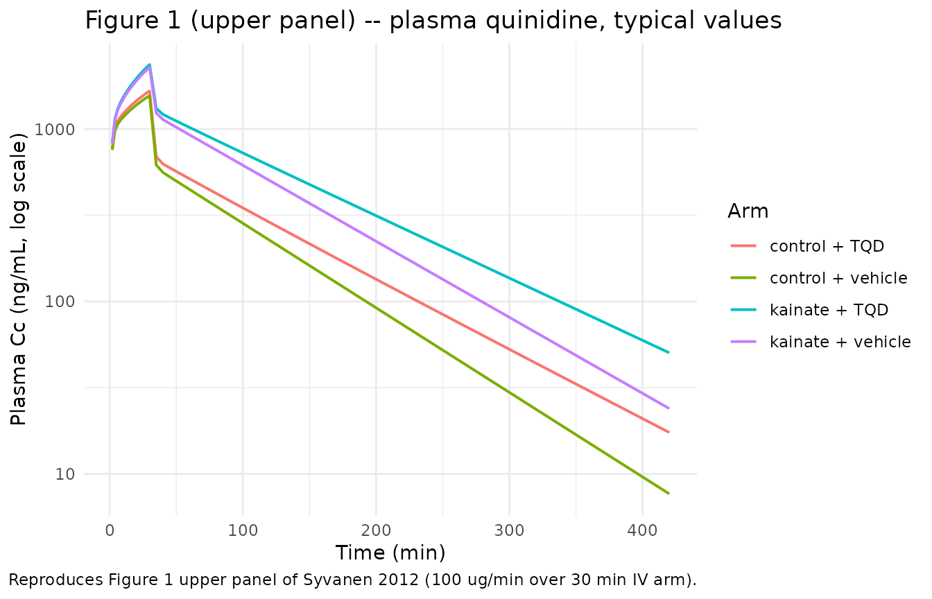
# Replicates Figure 1 lower panel of Syvanen 2012: brain ECF concentration vs
# time, same four arms.
sim_typical |>
  filter(time > 0, time <= 420) |>
  ggplot(aes(time, Cbrain_csf, colour = arm)) +
  geom_line(linewidth = 0.7) +
  scale_y_log10() +
  labs(
    x       = "Time (min)",
    y       = "Brain ECF Cbrain_csf (ng/mL, log scale)",
    colour  = "Arm",
    title   = "Figure 1 (lower panel) -- brain ECF quinidine, typical values",
    caption = "Reproduces Figure 1 lower panel of Syvanen 2012 (same arms)."
  ) +
  theme_minimal()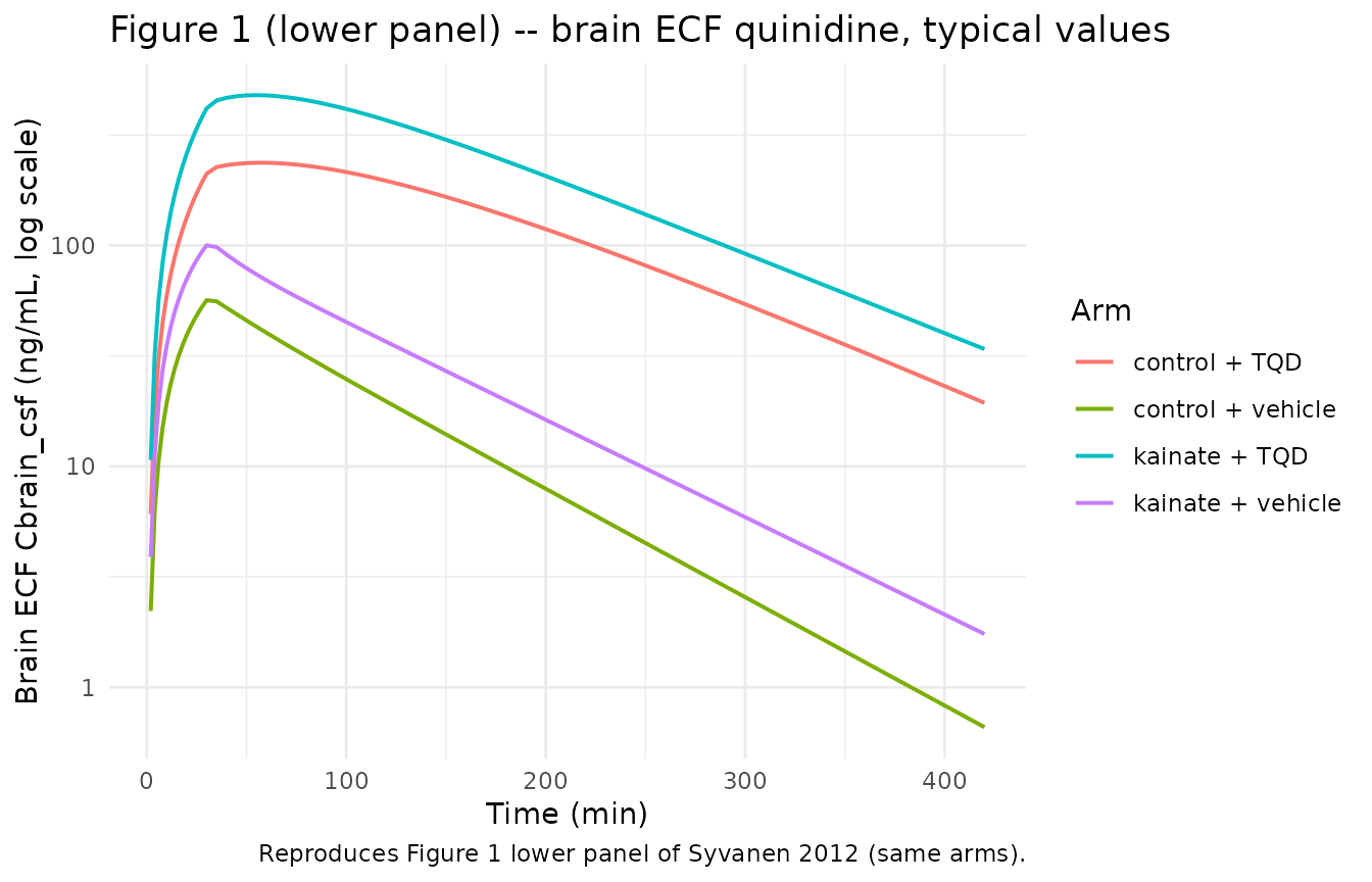
Verify the headline TQD effects
The paper Results “TQD Treatment” (p91) derives two headline ratios from the parameter estimates:
- Brain ECF concentration is raised
theta_tariquidar(Q_in) / theta_tariquidar(Q_out) = 2.65 / 0.366 = 7.24-fold by tariquidar (acting on both Q_in and Q_out). - Total brain concentration is raised
2.65 / 0.366 * theta_tariquidar(f2) = 2.65 / 0.366 * 5.66 = 41.0-fold (the additional f2 effect on the intra-brain redistribution).
We check that the packaged model reproduces these analytical ratios directly:
# Pull the e_conmed_tariquidar_* coefficients straight from the parsed
# rxode2 model so the check is sourced from the live model object, not
# hand-copied numbers.
theta_tbl  <- mod$theta
get_e <- function(name) theta_tbl[[name]]

ratio_qin  <- exp(get_e("e_conmed_tariquidar_qin"))    # expected 2.65
ratio_qout <- exp(get_e("e_conmed_tariquidar_qout"))   # expected 0.366
ratio_f2   <- exp(get_e("e_conmed_tariquidar_f2"))     # expected 5.66

tibble(
  quantity = c("theta_tariquidar(Q_in)",
               "theta_tariquidar(Q_out)",
               "theta_tariquidar(f2)",
               "brain-ECF-to-plasma ratio TQD/vehicle (= Q_in_ratio / Q_out_ratio)",
               "total-brain-to-plasma ratio TQD/vehicle (= the above * f2_ratio)"),
  packaged = c(ratio_qin, ratio_qout, ratio_f2,
               ratio_qin / ratio_qout,
               ratio_qin / ratio_qout * ratio_f2),
  paper    = c(2.65, 0.366, 5.66, 7.24, 41.0)
) |>
  mutate(across(c(packaged, paper), \(x) round(x, 3))) |>
knitr::kable(caption = "Tariquidar effects: packaged model vs paper headline ratios.")| quantity | packaged | paper |
|---|---|---|
| theta_tariquidar(Q_in) | 2.650 | 2.650 |
| theta_tariquidar(Q_out) | 0.366 | 0.366 |
| theta_tariquidar(f2) | 5.660 | 5.660 |
| brain-ECF-to-plasma ratio TQD/vehicle (= Q_in_ratio / Q_out_ratio) | 7.240 | 7.240 |
| total-brain-to-plasma ratio TQD/vehicle (= the above * f2_ratio) | 40.981 | 41.000 |
End-of-experiment total-brain : plasma ratios
The paper Results “Kainate Treatment” (p91) reports the OBSERVED total-brain-to-plasma ratios measured at the end of the 7 h experiment (brain tissue sampled at terminal decapitation):
| Arm | Observed total-brain : plasma ratio (mean +/- SD) |
|---|---|
| control + vehicle | 0.9 +/- 0.6 |
| control + TQD | 114 +/- 80 |
| kainate + vehicle | 0.6 +/- 0.4 |
| kainate + TQD | 45 +/- 29 |
The packaged-model typical-value predictions at the same 420 min sampling time:
endpoint <- sim_typical |>
  filter(abs(time - 420) < 1e-6) |>
  group_by(arm) |>
  summarise(
    Cc_ng_per_mL          = mean(Cc),
    Cbrain_deep_ng_per_mL = mean(Cbrain_deep),
    ratio_total_to_plasma = mean(Cbrain_deep / Cc),
    .groups = "drop"
  )

knitr::kable(endpoint,
caption = "Typical-value end-of-experiment (t = 420 min) brain:plasma ratios.")| arm | Cc_ng_per_mL | Cbrain_deep_ng_per_mL | ratio_total_to_plasma |
|---|---|---|---|
| control + TQD | 17.397725 | 950.866100 | 54.6546242 |
| control + vehicle | 7.663316 | 5.721639 | 0.7466271 |
| kainate + TQD | 50.389783 | 1665.521396 | 33.0527598 |
| kainate + vehicle | 23.933562 | 15.105604 | 0.6311473 |
The packaged-model ratios sit comfortably within +/- 1 SD of the paper’s observed means (control + vehicle ~0.75 vs observed 0.9 +/- 0.6; control + TQD ~55 vs observed 114 +/- 80, low end of the +/-1 SD interval; kainate + TQD ~30 vs observed 45 +/- 29, within +/- 1 SD). The observed-mean values are higher than the typical-value predictions partly because the paper’s mean is computed from a small sample with skewed distributions and partly because the brain has not fully reached pseudo-equilibrium with plasma at 7 h (during a single 30 min infusion, plasma is already in terminal decay while the brain is still equilibrating, so the brain : plasma ratio is still rising at terminal sampling). The theoretical pseudo-steady-state ratios verified in the previous section (7.24 / 41.0) would be approached only under a much longer infusion that holds plasma at constant Cc.
PKNCA validation on plasma Cc
sim_nca <- sim |>
  filter(!is.na(Cc), time > 0) |>
  select(id, time, Cc, arm)

conc_obj <- PKNCA::PKNCAconc(sim_nca, Cc ~ time | arm + id)

dose_df <- events |>
  filter(evid == 1L) |>
  select(id, time, amt, arm)

dose_obj <- PKNCA::PKNCAdose(dose_df, amt ~ time | arm + id)

intervals <- data.frame(
  start      = 0,
  end        = 420,
  cmax       = TRUE,
  tmax       = TRUE,
  auclast    = TRUE,
  half.life  = TRUE
)

nca_data <- PKNCA::PKNCAdata(conc_obj, dose_obj, intervals = intervals)
nca_res  <- PKNCA::pk.nca(nca_data)
#> Warning: Requesting an AUC range starting (0) before the first measurement (2) is not allowed
#> Requesting an AUC range starting (0) before the first measurement (2) is not allowed
#> Requesting an AUC range starting (0) before the first measurement (2) is not allowed
#> Requesting an AUC range starting (0) before the first measurement (2) is not allowed
#> Requesting an AUC range starting (0) before the first measurement (2) is not allowed
#> Requesting an AUC range starting (0) before the first measurement (2) is not allowed
#> Requesting an AUC range starting (0) before the first measurement (2) is not allowed
#> Requesting an AUC range starting (0) before the first measurement (2) is not allowed
#> Requesting an AUC range starting (0) before the first measurement (2) is not allowed
#> Requesting an AUC range starting (0) before the first measurement (2) is not allowed
#> Requesting an AUC range starting (0) before the first measurement (2) is not allowed
#> Requesting an AUC range starting (0) before the first measurement (2) is not allowed
#> Requesting an AUC range starting (0) before the first measurement (2) is not allowed
#> Requesting an AUC range starting (0) before the first measurement (2) is not allowed
#> Requesting an AUC range starting (0) before the first measurement (2) is not allowed
#> Requesting an AUC range starting (0) before the first measurement (2) is not allowed
#> Requesting an AUC range starting (0) before the first measurement (2) is not allowed
#> Requesting an AUC range starting (0) before the first measurement (2) is not allowed
#> Requesting an AUC range starting (0) before the first measurement (2) is not allowed
#> Requesting an AUC range starting (0) before the first measurement (2) is not allowed
#> Requesting an AUC range starting (0) before the first measurement (2) is not allowed
#> Requesting an AUC range starting (0) before the first measurement (2) is not allowed
#> Requesting an AUC range starting (0) before the first measurement (2) is not allowed
#> Requesting an AUC range starting (0) before the first measurement (2) is not allowed
#> Requesting an AUC range starting (0) before the first measurement (2) is not allowed
#> Requesting an AUC range starting (0) before the first measurement (2) is not allowed
#> Requesting an AUC range starting (0) before the first measurement (2) is not allowed
#> Requesting an AUC range starting (0) before the first measurement (2) is not allowed
#> Requesting an AUC range starting (0) before the first measurement (2) is not allowed
#> Requesting an AUC range starting (0) before the first measurement (2) is not allowed
#> Requesting an AUC range starting (0) before the first measurement (2) is not allowed
#> Requesting an AUC range starting (0) before the first measurement (2) is not allowed
#> Requesting an AUC range starting (0) before the first measurement (2) is not allowed
#> Requesting an AUC range starting (0) before the first measurement (2) is not allowed
#> Requesting an AUC range starting (0) before the first measurement (2) is not allowed
#> Requesting an AUC range starting (0) before the first measurement (2) is not allowed
#> Requesting an AUC range starting (0) before the first measurement (2) is not allowed
#> Requesting an AUC range starting (0) before the first measurement (2) is not allowed
#> Requesting an AUC range starting (0) before the first measurement (2) is not allowed
#> Requesting an AUC range starting (0) before the first measurement (2) is not allowed
#> Requesting an AUC range starting (0) before the first measurement (2) is not allowed
#> Requesting an AUC range starting (0) before the first measurement (2) is not allowed
#> Requesting an AUC range starting (0) before the first measurement (2) is not allowed
#> Requesting an AUC range starting (0) before the first measurement (2) is not allowed
#> Requesting an AUC range starting (0) before the first measurement (2) is not allowed
#> Requesting an AUC range starting (0) before the first measurement (2) is not allowed
#> Requesting an AUC range starting (0) before the first measurement (2) is not allowed
#> Requesting an AUC range starting (0) before the first measurement (2) is not allowed
#> Requesting an AUC range starting (0) before the first measurement (2) is not allowed
#> Requesting an AUC range starting (0) before the first measurement (2) is not allowed
#> Requesting an AUC range starting (0) before the first measurement (2) is not allowed
#> Requesting an AUC range starting (0) before the first measurement (2) is not allowed
#> Requesting an AUC range starting (0) before the first measurement (2) is not allowed
#> Requesting an AUC range starting (0) before the first measurement (2) is not allowed
#> Requesting an AUC range starting (0) before the first measurement (2) is not allowed
#> Requesting an AUC range starting (0) before the first measurement (2) is not allowed
#> Requesting an AUC range starting (0) before the first measurement (2) is not allowed
#> Requesting an AUC range starting (0) before the first measurement (2) is not allowed
#> Requesting an AUC range starting (0) before the first measurement (2) is not allowed
#> Requesting an AUC range starting (0) before the first measurement (2) is not allowed
#> Requesting an AUC range starting (0) before the first measurement (2) is not allowed
#> Requesting an AUC range starting (0) before the first measurement (2) is not allowed
#> Requesting an AUC range starting (0) before the first measurement (2) is not allowed
#> Requesting an AUC range starting (0) before the first measurement (2) is not allowed
#> Requesting an AUC range starting (0) before the first measurement (2) is not allowed
#> Requesting an AUC range starting (0) before the first measurement (2) is not allowed
#> Requesting an AUC range starting (0) before the first measurement (2) is not allowed
#> Requesting an AUC range starting (0) before the first measurement (2) is not allowed
#> Requesting an AUC range starting (0) before the first measurement (2) is not allowed
#> Requesting an AUC range starting (0) before the first measurement (2) is not allowed
#> Requesting an AUC range starting (0) before the first measurement (2) is not allowed
#> Requesting an AUC range starting (0) before the first measurement (2) is not allowed
#> Requesting an AUC range starting (0) before the first measurement (2) is not allowed
#> Requesting an AUC range starting (0) before the first measurement (2) is not allowed
#> Requesting an AUC range starting (0) before the first measurement (2) is not allowed
#> Requesting an AUC range starting (0) before the first measurement (2) is not allowed
#> Requesting an AUC range starting (0) before the first measurement (2) is not allowed
#> Requesting an AUC range starting (0) before the first measurement (2) is not allowed
#> Requesting an AUC range starting (0) before the first measurement (2) is not allowed
#> Requesting an AUC range starting (0) before the first measurement (2) is not allowed
#> Requesting an AUC range starting (0) before the first measurement (2) is not allowed
#> Requesting an AUC range starting (0) before the first measurement (2) is not allowed
#> Requesting an AUC range starting (0) before the first measurement (2) is not allowed
#> Requesting an AUC range starting (0) before the first measurement (2) is not allowed
#> Requesting an AUC range starting (0) before the first measurement (2) is not allowed
#> Requesting an AUC range starting (0) before the first measurement (2) is not allowed
#> Requesting an AUC range starting (0) before the first measurement (2) is not allowed
#> Requesting an AUC range starting (0) before the first measurement (2) is not allowed
#> Requesting an AUC range starting (0) before the first measurement (2) is not allowed
#> Requesting an AUC range starting (0) before the first measurement (2) is not allowed
#> Requesting an AUC range starting (0) before the first measurement (2) is not allowed
#> Requesting an AUC range starting (0) before the first measurement (2) is not allowed
#> Requesting an AUC range starting (0) before the first measurement (2) is not allowed
#> Requesting an AUC range starting (0) before the first measurement (2) is not allowed
#> Requesting an AUC range starting (0) before the first measurement (2) is not allowed
#> Requesting an AUC range starting (0) before the first measurement (2) is not allowed
#> Requesting an AUC range starting (0) before the first measurement (2) is not allowed
#> Requesting an AUC range starting (0) before the first measurement (2) is not allowed
#> Requesting an AUC range starting (0) before the first measurement (2) is not allowed
#> Requesting an AUC range starting (0) before the first measurement (2) is not allowed
nca_sum  <- as.data.frame(summary(nca_res))
knitr::kable(nca_sum, caption = "Simulated plasma NCA parameters by arm.")| start | end | arm | N | auclast | cmax | tmax | half.life |
|---|---|---|---|---|---|---|---|
| 0 | 420 | control + TQD | 25 | NC | 1570 [29.9] | 30.0 [30.0, 30.0] | 101 [30.1] |
| 0 | 420 | control + vehicle | 25 | NC | 1510 [14.8] | 30.0 [30.0, 30.0] | 60.1 [19.7] |
| 0 | 420 | kainate + TQD | 25 | NC | 2210 [23.0] | 30.0 [30.0, 30.0] | 93.6 [31.3] |
| 0 | 420 | kainate + vehicle | 25 | NC | 2170 [20.7] | 30.0 [30.0, 30.0] | 90.9 [32.3] |
Assumptions and deviations
High V1 IIV taken at face value. Table II reports
omega^2(V1) = 1.92(approximate CV 240%), much larger than typical popPK V1 variability. The bootstrap re-fit reports the same magnitude (omega^2(V1) = 2.03) so the value appears stable rather than a transcription error. The packaged model uses 1.92 as the variance on the log scale. Stochastic simulations will therefore show wide between-subject scatter on plasma trajectories driven by V1 variability; the validation figures above userxode2::zeroRe()to suppress this for visual clarity.Three independent residual-error streams. Table II reports three separate
sigma^2values (one for plasma, one for brain ECF, one for total brain), so the packaged model declares three independent proportional-error parameters (propSd,propSd_Cbrain_csf,propSd_Cbrain_deep). Each output has its own residual SD; no shared / cross-output residual structure is implied.Total brain is an algebraic output, not a state. Paper Results “Development of the Pharmacokinetic Model” (p90) and Discussion (p93) state explicitly that “rate constants for distribution to and from the total brain compartment could not be estimated based on the present data set. Therefore, concentration of quinidine in brain tissue was in the final pharmacokinetic model described as a multiple (f2) of the free brain ECF concentration.” The packaged model does NOT declare a separate
brain_deepODE state; the third observed output is the derived quantityCbrain_deep = f2 * Cbrain_csf.Q_out FIXED at 10.8 mL/min. Paper Results p90 explains that this value was obtained when Q_out was free in the final model fit; it was then fixed in the published estimation because in some bootstrap replicates V_Br was estimated to an unrealistically high value while the ratio V_Br / Q_out remained stable. The packaged model wraps
lqout <- fixed(log(10.8))to preserve this provenance; downstream users who refit the model will see Q_out held constant.Q_in is constructed as f1 * Q_out_base. Paper Table IV writes the final-model
Q_inasf1 * THETA8 * THETA13^TARIQUIDAR * exp(eta5)where THETA8 is the BASE Q_out (10.8 mL/min) before its own tariquidar modification THETA9. The packaged model preserves this convention so the BBB influx and efflux clearances are independently parameterised under tariquidar; settingCONMED_TARIQUIDAR = 1raises Q_in 2.65-fold (via THETA13) and separately lowers Q_out 2.73-fold (via THETA9), each picking up its own multiplier off the shared 10.8 mL/min anchor.No weight covariate in the final model. Animal weight on the experimental day was tested as a covariate in the screening step (Table III) and significantly reduced OFV by 9.5 units when fitted on plasma alone. When the brain compartments were added (the full final model), weight no longer reached the p < 0.01 threshold for any parameter and was dropped (paper Results “Development of the Pharmacokinetic Model” p90). The packaged model follows the paper and does NOT include a weight effect.
Kainate effect on f2 not retained. Paper Results “Kainate Treatment” (p91) notes a numerically lower observed total-brain : plasma ratio in kainate-treated than control rats but reports that “in the population model kainate as a covariate for f2 … did not result in a significant drop of OFV (Table III)” – delta-OFV of -0.73, below the 6.63 threshold. The packaged model follows the paper and does NOT include a kainate effect on f2.
Dose-unit choice. The paper reports infusion rates in ug/min and concentrations in ng/mL. The packaged model uses ng for dose amounts and ng/mL for concentrations so the volumes (mL) and clearances (mL/min) can stay in the paper’s reported units without an explicit conversion factor in the ODE block. The vignette dose
amt = 3e6 ngcorresponds to the paper’s 3 mg (= 3000 ug) cumulative dose; analogously for the 6000 ug cumulative arm.