Oxaliplatin in rats with acute kidney injury (Kobuchi 2021)
Source:vignettes/articles/Kobuchi_2021_oxaliplatin_rat.Rmd
Kobuchi_2021_oxaliplatin_rat.RmdModel and source
- Citation: Kobuchi S, Kai M, Ito Y. Population Pharmacokinetic Model-Based Evaluation of Intact Oxaliplatin in Rats with Acute Kidney Injury. Cancers (Basel). 2021;13(24):6382. doi:10.3390/cancers13246382 (PMCID PMC8699120).
- Description: Preclinical (rat). Two-compartment population PK model with linear elimination for intact (unbiotransformed) oxaliplatin in plasma after a single intravenous bolus of 3 or 8 mg/kg to male Wistar rats with normal renal function or mild / severe acute kidney injury induced by 30 / 60 min renal ischemia-reperfusion (Kobuchi 2021). Parameters are per kg body weight (dose in mg/kg), exponential IIV on the central volume, clearance and intercompartmental clearance, proportional residual error. The final model carries no covariates: the paper’s renal-function simulation (Figure 5) substituted a post hoc clearance-versus-plasma-creatinine regression whose coefficients are not printed (see the vignette).
- Article: https://doi.org/10.3390/cancers13246382 (open access, PMC8699120)
- Supplement: https://www.mdpi.com/article/10.3390/cancers13246382/s1 (Figure S1, goodness-of-fit plots only; no parameter values)
Kobuchi 2021 measured intact oxaliplatin (L-OHP, not total platinum) by LC-MS/MS in rat plasma and fitted a two-compartment population PK model in Phoenix NLME 8.2 (FOCE-ELS). The model was then used to simulate exposure over a range of plasma creatinine values to ask whether oxaliplatin needs a dose reduction in acute kidney injury (AKI).
Population
Thirty 10-week-old male Wistar rats (about 300 g) were split into normal, mild-AKI and severe-AKI groups. AKI was induced by clamping both renal arteries for 30 min (mild) or 60 min (severe) followed by 24 h of reperfusion; controls had sham surgery. Each renal-function group received a single intravenous bolus of oxaliplatin (Elplat) at 3 or 8 mg/kg into the jugular vein (n = 5 per dose group). Plasma was sampled at 3, 5, 10, 20, 30 and 45 min and 1, 1.5 and 2 h. Table 1 of the paper gives mean (SD) plasma creatinine of 0.27 (0.02), 0.54 (0.21) and 0.95 (0.17) mg/dL and creatinine clearance of 4.2 (1.3), 2.2 (0.7) and 1.6 (0.7) mL/min/kg in the normal, mild and severe groups.
The same information is available programmatically via
readModelDb("Kobuchi_2021_oxaliplatin_rat")()$population.
Source trace
Every ini() value carries an in-file comment in
inst/modeldb/specificDrugs/Kobuchi_2021_oxaliplatin_rat.R.
They are collected here.
| Equation / parameter | Value | Source location |
|---|---|---|
| Two-compartment, linear elimination, IV bolus | n/a | Section 2.4 and Section 3.3 (“A two-compartment model with a linear elimination”) |
lvc (V) |
log(0.44) L/kg | Table 3, fixed effects |
lvp (V2) |
log(2.26) L/kg | Table 3, fixed effects |
lcl (CL) |
log(1.76) L/h/kg | Table 3, fixed effects |
lq (CL2) |
log(1.0) L/h/kg | Table 3, fixed effects |
etalvc |
0.375^2 = 0.140625 | Table 3, IIV on V = 37.5% |
etalcl |
0.305^2 = 0.093025 | Table 3, IIV on CL = 30.5% |
etalq |
0.315^2 = 0.099225 | Table 3, IIV on CL2 = 31.5% |
| Exponential IIV | n/a | Section 2.4 (“assumed by the exponential error model”) |
propSd |
0.149 | Table 3, residual variability C = 14.9%; proportional per Section 2.4 |
Cc <- central / vc |
n/a | Plasma concentration in the central compartment (Table 3 footnote, C) |
The text of Section 3.3 restates the estimates: V and V2 of 0.44 and 2.26 L/kg (sum 2.70 L/kg), CL of 1.76 and CL2 of 1.0 L/h/kg. The paper’s “CLtot: 2.76 L/h/kg” is the arithmetic sum CL + CL2; it is not a model quantity (total clearance of the model is CL alone).
mod <- readModelDb("Kobuchi_2021_oxaliplatin_rat")
ui <- rxode2::rxode(mod)
#> ℹ parameter labels from comments will be replaced by 'label()'
th <- ui$theta
stopifnot(
  abs(exp(th[["lvc"]]) + exp(th[["lvp"]]) - 2.70) < 1e-8, # Section 3.3 'Vd: 2.70 L/kg'
  abs(exp(th[["lcl"]]) + exp(th[["lq"]]) - 2.76) < 1e-8 #   Section 3.3 'CLtot: 2.76 L/h/kg'
)
Typical-value check
For a linear model after an IV bolus,
AUC(0-inf) = Dose / CL exactly, so the typical rat must
give 3 / 1.76 = 1.705 and 8 / 1.76 = 4.545 ug*h/mL. The solve below uses
a log-spaced grid out to 72 h, which leaves a negligible extrapolated
tail.
mod_typ <- rxode2::zeroRe(mod)
#> ℹ parameter labels from comments will be replaced by 'label()'
tgrid <- sort(unique(c(0, exp(seq(log(0.005), log(72), length.out = 400)))))
ev_typ <- dplyr::bind_rows(
  data.frame(id = 1L, time = 0, amt = 3, evid = 1L, cmt = "central", dose = 3),
  data.frame(id = 1L, time = tgrid, amt = 0, evid = 0L, cmt = "central", dose = 3),
  data.frame(id = 2L, time = 0, amt = 8, evid = 1L, cmt = "central", dose = 8),
  data.frame(id = 2L, time = tgrid, amt = 0, evid = 0L, cmt = "central", dose = 8)
)
sim_typ <- rxode2::rxSolve(mod_typ, events = ev_typ, keep = "dose") |>
  as.data.frame()
#> ℹ omega/sigma items treated as zero: 'etalvc', 'etalcl', 'etalq'
#> Warning: multi-subject simulation without without 'omega'

typ_nca <- sim_typ |>
  dplyr::group_by(dose) |>
  dplyr::summarise(
    auc = sum(diff(time) * (head(Cc, -1) + tail(Cc, -1)) / 2) +
      dplyr::last(Cc) / (log(Cc[n() - 1] / Cc[n()]) / (time[n()] - time[n() - 1])),
    cl = dplyr::first(cl),
    .groups = "drop"
  ) |>
  dplyr::mutate(expected = dose / cl, pct_diff = 100 * (auc / expected - 1))
knitr::kable(typ_nca, digits = 3, caption = "Typical-value AUC(0-inf) against Dose / CL.")| dose | auc | cl | expected | pct_diff |
|---|---|---|---|---|
| 3 | 1.705 | 1.76 | 1.705 | 0.01 |
| 8 | 4.546 | 1.76 | 4.545 | 0.01 |
Virtual cohort and simulation
Two dose arms of 200 virtual rats each, sampled at the paper’s nine plasma times plus a time-zero row (the IV-bolus initial concentration).
rxode2::rxSetSeed(20211220)
paper_times <- c(3, 5, 10, 20, 30, 45, 60, 90, 120) / 60
make_arm <- function(n, dose, id_offset) {
  ids <- id_offset + seq_len(n)
  dplyr::bind_rows(
    data.frame(id = ids, time = 0, amt = dose, evid = 1L, cmt = "central"),
    tidyr::expand_grid(id = ids, time = c(0, paper_times)) |>
      dplyr::mutate(amt = 0, evid = 0L, cmt = "central")
  ) |>
    dplyr::mutate(treatment = paste(dose, "mg/kg")) |>
    dplyr::arrange(id, time, dplyr::desc(evid))
}
events <- dplyr::bind_rows(
  make_arm(200, 3, 0L),
  make_arm(200, 8, 200L)
)
stopifnot(!anyDuplicated(unique(events[, c("id", "time", "evid")])))

sim <- rxode2::rxSolve(mod, events = events, keep = "treatment") |>
  as.data.frame()
#> ℹ parameter labels from comments will be replaced by 'label()'
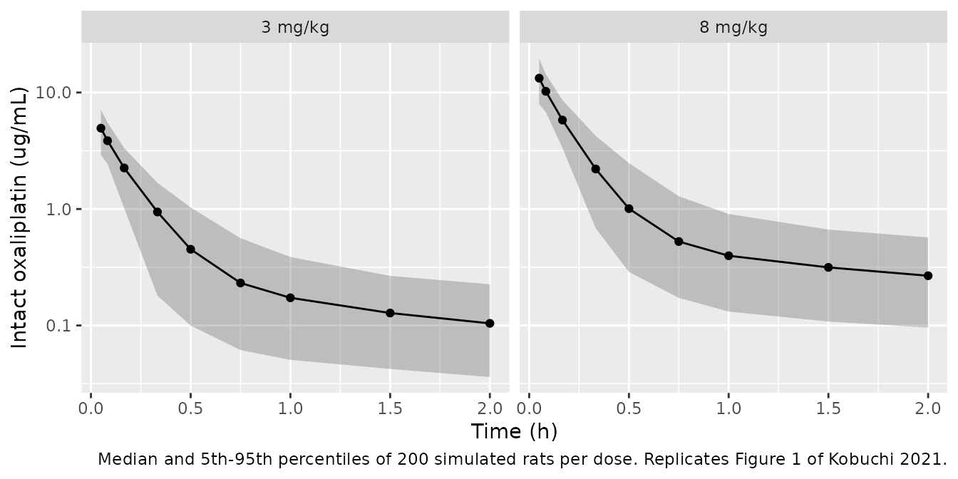
Replicate Figure 1
# Replicates Figure 1 of Kobuchi 2021: plasma intact oxaliplatin after 3 or
# 8 mg/kg IV. The paper plots mean +/- SD per renal-function group; the model
# has no renal-function covariate, so one pooled band is shown per dose.
sim |>
  dplyr::filter(time > 0) |>
  dplyr::group_by(treatment, time) |>
  dplyr::summarise(
    Q05 = quantile(Cc, 0.05), Q50 = median(Cc), Q95 = quantile(Cc, 0.95),
    .groups = "drop"
  ) |>
  ggplot(aes(time, Q50)) +
  geom_ribbon(aes(ymin = Q05, ymax = Q95), alpha = 0.25) +
  geom_line() +
  geom_point() +
  facet_wrap(~treatment) +
  scale_y_log10() +
  labs(
    x = "Time (h)", y = "Intact oxaliplatin (ug/mL)",
    caption = "Median and 5th-95th percentiles of 200 simulated rats per dose. Replicates Figure 1 of Kobuchi 2021."
  )
PKNCA validation
Kobuchi 2021 ran NCA in Phoenix WinNonlin with the linear trapezoidal rule on the 0-2 h profiles; PKNCA is set to the same rule. The published Table 2 means are per renal-function group, so the reference below is the unweighted mean of the three group means at each dose (all groups had n = 4-5).
sim_nca <- sim |>
  dplyr::filter(!is.na(Cc)) |>
  dplyr::select(id, time, Cc, treatment)

dose_df <- events |>
  dplyr::filter(evid == 1) |>
  dplyr::select(id, time, amt, treatment)

conc_obj <- PKNCA::PKNCAconc(sim_nca, Cc ~ time | treatment + id)
dose_obj <- PKNCA::PKNCAdose(dose_df, amt ~ time | treatment + id, route = "intravascular")
intervals <- data.frame(
  start = 0, end = Inf,
  aucinf.obs = TRUE, half.life = TRUE, cl.obs = TRUE, vz.obs = TRUE
)
nca_res <- PKNCA::pk.nca(PKNCA::PKNCAdata(
  conc_obj, dose_obj,
  intervals = intervals,
  options = list(auc.method = "linear")
))

# Table 2 of Kobuchi 2021, mean over the normal / mild / severe group means.
published <- tibble::tribble(
  ~treatment, ~aucinf.obs, ~half.life, ~cl.obs, ~vz.obs,
  "3 mg/kg", mean(c(2.0, 2.2, 2.4)), mean(c(2.6, 2.8, 2.3)), mean(c(1.6, 1.4, 1.3)), mean(c(5.8, 5.7, 3.8)),
  "8 mg/kg", mean(c(3.4, 3.3, 4.4)), mean(c(0.7, 0.7, 0.9)), mean(c(2.5, 2.2, 1.9)), mean(c(2.4, 2.9, 2.2))
)

cmp <- nlmixr2lib::ncaComparisonTable(
  simulated = nca_res,
  reference = published,
  by = "treatment",
  units = c(aucinf.obs = "ug*h/mL", half.life = "h", cl.obs = "L/h/kg", vz.obs = "L/kg"),
  tolerance_pct = 20
)
knitr::kable(
  cmp,
  caption = "Simulated (median) vs. published NCA (Table 2, mean of the three renal-function groups). * differs by >20%."
)| NCA parameter | treatment | Reference | Simulated | % diff |
|---|---|---|---|---|
| AUC0-∞ (obs) (ug*h/mL) | 3 mg/kg | 2.2 | 1.58 | -28.4%* |
| AUC0-∞ (obs) (ug*h/mL) | 8 mg/kg | 3.7 | 4.18 | +12.9% |
| t½ (h) | 3 mg/kg | 2.57 | 1.86 | -27.5%* |
| t½ (h) | 8 mg/kg | 0.767 | 1.94 | +152.5%* |
| CL/F (L/h/kg) | 3 mg/kg | 1.43 | 1.9 | +32.8%* |
| CL/F (L/h/kg) | 8 mg/kg | 2.2 | 1.91 | -13.0% |
| Vz/F (L/kg) | 3 mg/kg | 5.1 | 4.63 | -9.2% |
| Vz/F (L/kg) | 8 mg/kg | 2.5 | 4.96 | +98.6%* |
The model is one pooled fit across both doses and all three
renal-function groups, and Table 2 itself is not dose-proportional:
dose-normalised AUC is 0.67-0.80 at 3 mg/kg and 0.41-0.55 at 8 mg/kg
(h*kg/L), while the linear model gives a single 1 / CL = 0.57 for both.
The simulated AUC therefore falls below the 3 mg/kg groups and inside
the range of the 8 mg/kg groups, with clearance mirroring it. (NCA on
the 0-2 h window also puts the simulated median AUC a little under Dose
/ CL, because the terminal slope fitted inside 2 h is steeper than the
model’s true terminal phase, whose half-life is about 2.5 h.) The
half-life and volume differ most at 8 mg/kg, where the published
half-life of 0.7-0.9 h is far shorter than at 3 mg/kg on the same
sampling schedule; the authors attribute the difference to sampling, and
the pooled linear model cannot reproduce it.
ncaComparisonTable() labels the clearance and volume rows
“CL/F” and “Vz/F”; after an IV bolus they are CL and Vz. The paper
states only that its model values are “comparable with” / “similar to”
the NCA values, which is what the check below asserts.
# Structural checks the paper itself states (Section 3.3): the model CL lies
# within the NCA CLtot range 1.3-2.5 L/h/kg, the model V + V2 lies within the
# NCA Vd range 2.2-5.8 L/kg, and the typical dose-normalised AUC lies between
# the published 3 mg/kg and 8 mg/kg group means.
cl_typ <- exp(th[["lcl"]])
dn_auc_pub <- c(c(2.0, 2.2, 2.4) / 3, c(3.4, 3.3, 4.4) / 8)
stopifnot(
  cl_typ > 1.3, cl_typ < 2.5,
  exp(th[["lvc"]]) + exp(th[["lvp"]]) > 2.2,
  exp(th[["lvc"]]) + exp(th[["lvp"]]) < 5.8,
  1 / cl_typ > min(dn_auc_pub), 1 / cl_typ < max(dn_auc_pub)
)
Replicate Figure 5: exposure against plasma creatinine
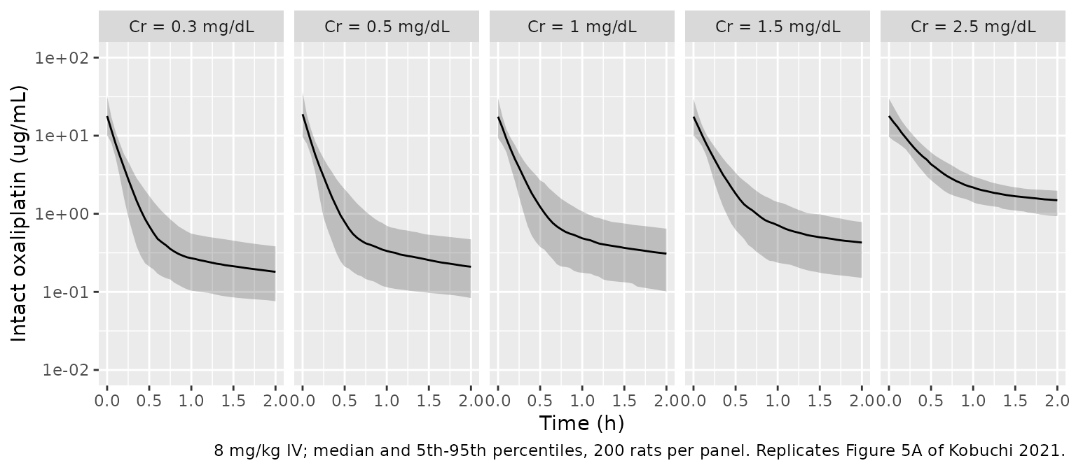
Section 2.5 simulates 8 mg/kg IV with CL “determined by the
regression equations of Cr level and post hoc CL” over plasma creatinine
0.3-2.5 mg/dL, and Section 3.4 prints the median (5th-95th percentile)
AUC(0-inf) at five creatinine values. The regression coefficients
themselves are not printed. Because AUC(0-inf) = Dose / CL
for this model, each published median fixes the typical clearance at
that creatinine: CL(Cr) = 8 / median AUC. The five
back-solved clearances fall on a straight line, so the maintainers take
the paper’s regression to be linear, CL = a + b * Cr, and
fit it here.
fig5 <- tibble::tribble(
  ~CREAT, ~auc_med, ~auc_p05, ~auc_p95,
  0.3, 3.4, 2.2, 5.3,
  0.5, 3.7, 2.4, 5.7,
  1.0, 4.6, 3.0, 7.2,
  1.5, 6.3, 4.1, 9.8,
  2.5, 21.7, 13.8, 42.5
) |>
  dplyr::mutate(cl_backsolved = 8 / auc_med)

fit5 <- lm(cl_backsolved ~ CREAT, data = fig5)
fit4 <- lm(cl_backsolved ~ CREAT, data = fig5[fig5$CREAT < 2.5, ])
fig5 <- fig5 |>
  dplyr::mutate(
    cl_fit = unname(predict(fit5, newdata = fig5)),
    pct_resid = 100 * (cl_fit / cl_backsolved - 1)
  )
auc25_from_fit4 <- 8 / unname(predict(fit4, newdata = data.frame(CREAT = 2.5)))
knitr::kable(
  fig5 |> dplyr::select(CREAT, auc_med, cl_backsolved, cl_fit, pct_resid),
  digits = 3,
  caption = "Clearance back-solved from each published median AUC and the linear fit."
)| CREAT | auc_med | cl_backsolved | cl_fit | pct_resid |
|---|---|---|---|---|
| 0.3 | 3.4 | 2.353 | 2.353 | 0.010 |
| 0.5 | 3.7 | 2.162 | 2.173 | 0.503 |
| 1.0 | 4.6 | 1.739 | 1.723 | -0.947 |
| 1.5 | 6.3 | 1.270 | 1.272 | 0.194 |
| 2.5 | 21.7 | 0.369 | 0.372 | 0.789 |
coef(fit5)
#> (Intercept)       CREAT
#>   2.6233909  -0.9007269
auc25_from_fit4
#> [1] 20.95816
# A straight line in Cr must reproduce all five back-solved clearances; this
# is what licenses the linear form. Held-out check: the line through the four
# Cr <= 1.5 points predicts the Cr = 2.5 median (21.7 ug*h/mL) to within 5%
# (it is the most leveraged point: CL falls to about 0.37 L/h/kg there).
stopifnot(
  all(abs(fig5$pct_resid) < 2),
  abs(auc25_from_fit4 / 21.7 - 1) < 0.05
)
The fitted line gives CL = 2.623 + (-0.901) x Cr L/h/kg. At the normal-group creatinine of 0.27 mg/dL this is about 2.38 L/h/kg, higher than the population estimate of 1.76 L/h/kg in Table 3, as expected for a regression on post hoc clearances rather than on the population typical value.
The simulation below keeps every Table 3 parameter except the typical
CL, which is replaced by the fitted CL(Cr); the Table 3 IIV
on CL is applied on top.
cr_levels <- fig5$CREAT
ev5 <- dplyr::bind_rows(lapply(seq_along(cr_levels), function(i) {
  make_arm(200, 8, (i - 1L) * 200L) |>
    dplyr::mutate(CREAT = cr_levels[i])
})) |>
  dplyr::select(-treatment)
# Replace the dense 0-2 h grid for the plot.
ev5 <- dplyr::bind_rows(
  ev5 |> dplyr::filter(evid == 1),
  tidyr::expand_grid(
    ev5 |> dplyr::distinct(id, CREAT),
    time = seq(0, 2, by = 0.05)
  ) |>
    dplyr::mutate(amt = 0, evid = 0L, cmt = "central")
) |>
  dplyr::arrange(id, time, dplyr::desc(evid))
stopifnot(!anyDuplicated(unique(ev5[, c("id", "time", "evid")])))

sim5 <- dplyr::bind_rows(lapply(cr_levels, function(cr) {
  cl_cr <- unname(predict(fit5, newdata = data.frame(CREAT = cr)))
  rxode2::rxSolve(
    mod,
    events = ev5[ev5$CREAT == cr, ],
    params = c(lcl = log(cl_cr)),
    keep = "CREAT"
  ) |>
    as.data.frame()
}))

sim5 |>
  dplyr::group_by(CREAT, time) |>
  dplyr::summarise(
    Q05 = quantile(Cc, 0.05), Q50 = median(Cc), Q95 = quantile(Cc, 0.95),
    .groups = "drop"
  ) |>
  dplyr::mutate(panel = paste("Cr =", CREAT, "mg/dL")) |>
  ggplot(aes(time, Q50)) +
  geom_ribbon(aes(ymin = Q05, ymax = Q95), alpha = 0.25) +
  geom_line() +
  facet_wrap(~panel, nrow = 1) +
  scale_y_log10(limits = c(0.01, 100)) +
  labs(
    x = "Time (h)", y = "Intact oxaliplatin (ug/mL)",
    caption = "8 mg/kg IV; median and 5th-95th percentiles, 200 rats per panel. Replicates Figure 5A of Kobuchi 2021."
  )
# AUC(0-inf) per rat is exactly Dose / individual CL for this linear model.
auc5 <- sim5 |>
  dplyr::distinct(id, CREAT, cl) |>
  dplyr::mutate(auc = 8 / cl) |>
  dplyr::group_by(CREAT) |>
  dplyr::summarise(
    sim_med = median(auc), sim_p05 = quantile(auc, 0.05), sim_p95 = quantile(auc, 0.95),
    .groups = "drop"
  ) |>
  dplyr::left_join(fig5 |> dplyr::select(CREAT, auc_med, auc_p05, auc_p95), by = "CREAT") |>
  dplyr::mutate(pct_diff_med = 100 * (sim_med / auc_med - 1))

auc5 |>
  dplyr::rename(
    "Cr (mg/dL)" = CREAT,
    "Simulated median" = sim_med, "Simulated 5th" = sim_p05, "Simulated 95th" = sim_p95,
    "Published median" = auc_med, "Published 5th" = auc_p05, "Published 95th" = auc_p95,
    "Median % diff" = pct_diff_med
  ) |>
knitr::kable(digits = 2, caption = "AUC(0-inf) (ug*h/mL) after 8 mg/kg by plasma creatinine; published values from Section 3.4 (Figure 5B).")| Cr (mg/dL) | Simulated median | Simulated 5th | Simulated 95th | Published median | Published 5th | Published 95th | Median % diff |
|---|---|---|---|---|---|---|---|
| 0.3 | 3.47 | 2.04 | 5.28 | 3.4 | 2.2 | 5.3 | 1.98 |
| 0.5 | 3.73 | 2.40 | 6.07 | 3.7 | 2.4 | 5.7 | 0.72 |
| 1.0 | 4.62 | 2.76 | 7.49 | 4.6 | 3.0 | 7.2 | 0.36 |
| 1.5 | 6.24 | 3.54 | 9.94 | 6.3 | 4.1 | 9.8 | -0.98 |
| 2.5 | 20.68 | 13.05 | 34.34 | 21.7 | 13.8 | 42.5 | -4.69 |
# The medians are close to the published values by construction (the line was
# fitted to them); with 200 rats the sampling SE of a median is about 2.7% in
# log terms, so a 10% bound fails only if the CL(Cr) override did not reach
# the solve (every panel would then sit at 8 / 1.76 = 4.5 ug*h/mL, 79% off at
# Cr = 2.5) or the IIV is centred wrongly.
stopifnot(all(abs(auc5$pct_diff_med) < 10))
# Replicates Figure 5B of Kobuchi 2021 (AUC by creatinine), with the published
# median and 5th-95th percentiles overlaid in red.
sim5 |>
  dplyr::distinct(id, CREAT, cl) |>
  dplyr::mutate(auc = 8 / cl) |>
  ggplot(aes(factor(CREAT), auc)) +
  geom_boxplot(outlier.size = 0.5) +
  geom_pointrange(
    data = fig5,
    aes(x = factor(CREAT), y = auc_med, ymin = auc_p05, ymax = auc_p95),
    colour = "red", position = position_nudge(x = 0.3), inherit.aes = FALSE
  ) +
  scale_y_log10() +
  labs(
    x = "Plasma creatinine (mg/dL)", y = "AUC(0-inf) (ug*h/mL)",
    caption = "Simulated (boxes) vs. published median and 5th-95th percentiles (red). Replicates Figure 5B of Kobuchi 2021."
  )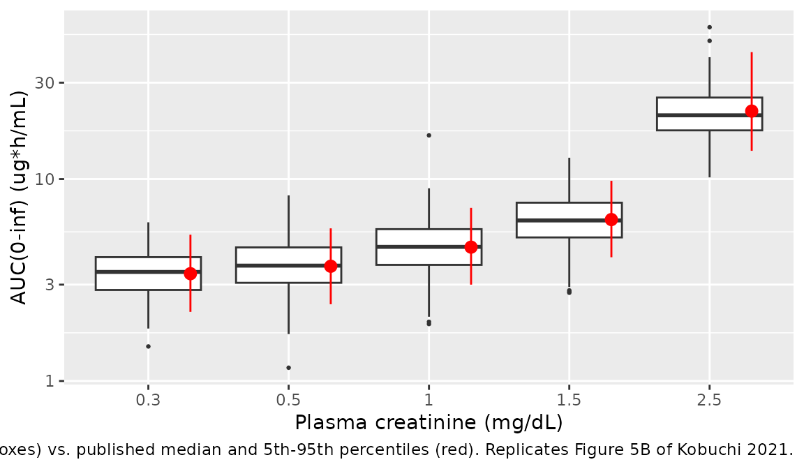
For Cr of 0.3-1.5 mg/dL each published 5th-95th percentile band spans a factor of about 2.4, a log-scale SD of about 0.27. The Table 3 IIV on CL of 30.5% gives 0.305 under the omega x 100 reading used here and 0.298 under the lognormal-CV reading. Both are a little wider than the published band, and they differ from each other by far less than the sampling noise in a 5th or 95th percentile, so the band cannot choose between the two readings. At Cr = 2.5 mg/dL the published band is wider and skewed upward (upper limit 42.5 against a median of 21.7), which suggests the paper computed AUC(0-inf) by NCA on the simulated 0-2 h profiles, where the extrapolated tail dominates once CL is this low. The percentile bands are recorded as a known deviation and are not asserted.
Assumptions and deviations
-
IIV scale. Table 3 gives the IIV as a bare
percentage under the heading “Inter-individual variability (omega)”. The
maintainers read the percentages as omega x 100 (omega^2 = 0.375^2,
0.305^2 and 0.315^2), the convention the same group’s Phoenix NLME
tables were shown to use for dapagliflozin
(
Kobuchi_2025_dapagliflozin, where a published simulated percentile band separated the two readings). The lognormal-CV reading, omega^2 = log(1 + CV^2), gives 0.1316, 0.0889 and 0.0945: under 7% less variance and not distinguishable with the data printed in this paper (see the Figure 5 band discussion above). The IIV rows’ “CV%” column (19.3, 26.0, 18.7) is the precision of the estimate, not the IIV. -
No renal-function covariate in the packaged model.
Table 3 is the final estimated model and has no covariate. The
creatinine dependence shown in Figure 5 comes from a separate regression
of post hoc CL on creatinine whose coefficients are not printed. The
maintainers back-solved a linear
CL(Cr)from the five published median AUC values in the Figure 5 chunk above; it lives only in this vignette, and plasma creatinine is documented in the model’scovariatesDataExcluded. -
Per-kg parameterisation. The model is in L/kg and
L/h/kg, as published; supply the dose in mg/kg and read
Ccin ug/mL (mg/L). - Pooled NCA reference. The model has no dose or renal-function effect, so the Table 2 comparison uses the mean of the three renal-function group means at each dose.
- Urinary excretion not modelled. Cumulative urinary excretion of intact oxaliplatin (Figure 2) was below 0.1% of the dose and was not part of the population model.
- Figure 4 (pcVPC) not reproduced. Individual observed data are not published; Figure 1 is reproduced instead as the simulated profile check.
- No erratum or correction notice for this article was found on the publisher page or in Europe PMC as of 2026-09-30.