Model and source
- Citation: Wang X, Owzar K, Gupta P, Larson RA, Mulkey F, Miller AA, Lewis LD, Hurd D, Vij R, Ratain MJ, Murry DJ; for the Alliance for Clinical Trials in Oncology. Vatalanib population pharmacokinetics in patients with myelodysplastic syndrome: CALGB 10105 (Alliance). Br J Clin Pharmacol. 2014;78(5):1005-1013.
- Article: https://doi.org/10.1111/bcp.12427
- Source files on disk:
from_people/literature_2018_search/Wang_2014_Vatalanib_population_pharmacokinetics_in_87914e.pdf.
The packaged model Wang_2014_vatalanib is a
one-compartment open model with lagged first-order absorption and a
first-order auto-induction term on apparent oral clearance. Vatalanib is
an oral anti-angiogenic VEGFR tyrosine-kinase inhibitor; the paper
reinforces autoinduction of vatalanib metabolism (most plausibly via
CYP3A4) and quantifies the resulting time-dependent change in oral
clearance over the first week of therapy.
Population
The published model was fit to 137 adults with primary or therapy-related myelodysplastic syndrome enrolled in the Cancer and Leukemia Group B (CALGB) 10105 study (Alliance), a multicentre open-label phase II trial (86 male / 51 female; median age 70 years, range 20-91; median weight 80 kg, range 48-128; 128 Caucasian / 9 Other). Patients received 750 or 1250 mg oral vatalanib once daily in 28-day cycles; the protocol was amended after enrolment began to allow a 750 mg starting dose. Sampling was sparse: 564 plasma concentration measurements across 137 patients, with 66.5% within 24 h of the first dose (predose, 15-45 min, 1-3 h, 4-6 h), 26.6% between days 7-14, and 6.9% on day 28 (pre-cycle-2 trough) (Wang 2014 Methods ‘Pharmacokinetic sampling schedule’, p. 1006; demographics Table 1, p. 1008).
The structured demographics are also embedded in the model file as a
population list
(inst/modeldb/specificDrugs/Wang_2014_vatalanib.R)
alongside the covariatesDataExcluded register of
screened-but-not- retained covariates.
Source trace
The per-parameter origin is recorded as an in-file comment next to
each ini() entry in
inst/modeldb/specificDrugs/Wang_2014_vatalanib.R. The table
below collects them in one place for review.
| Equation / parameter | Value | Source location |
|---|---|---|
| Structural form: 1-compartment with lagged first-order absorption | n/a | Wang 2014 Methods ‘Base model building’ and Results ‘Model development’, pp. 1006-1008 |
Time-dependent CL:
CL/F(t) = CL_induced/F - delta_CL/F * exp(-K_induct * t)
|
n/a | Wang 2014 Methods ‘Base model building’ p. 1006; Results ‘Model development’ p. 1008 |
lcl_ss -> exp = 54.9 L/h (CL_induced/F) |
54.9 | Table 2 row ‘CL_induced/F’, p. 1009 (95% CI 42.5-67.2; 11.7% RSE) |
lcl_time -> exp = 30.1 L/h (delta_CL/F) |
30.1 | Table 2 row ‘delta_CL/F’, p. 1009 (95% CI 14.8-45.4; 27.6% RSE) |
lkdes -> exp = 0.023 /h (K_induct, fixed) |
0.023 | Table 2 row ‘K_induct’, p. 1009 (fixed; footnote * ‘maximal clearance induction was reached on day 7’) |
lvc -> exp = 53.8 L (Vd/F) |
53.8 | Table 2 row ‘Vd/F’, p. 1009 (95% CI 38.4-69.1; 14.9% RSE) |
lka -> exp = 0.172 /h (Ka) |
0.172 | Table 2 row ‘Ka’, p. 1009 (95% CI 0.141-0.203; 9.2% RSE) |
ltlag -> exp = 0.178 h (A_lag) |
0.178 | Table 2 row ‘A_lag’, p. 1009 (95% CI 0.136-0.220; 11.7% RSE) |
etalcl_ss IIV (CV 22.8%; omega^2 = log(1+0.228^2) =
0.0507) |
0.0507 | Table 2 row ‘IIV for CL_induced/F’, p. 1009 |
etalvc IIV (CV 84.4%; omega^2 = log(1+0.844^2) =
0.5380) |
0.5380 | Table 2 row ‘IIV for Vd/F’, p. 1009 |
etalka IIV (CV 35.4%; omega^2 = log(1+0.354^2) =
0.1181) |
0.1181 | Table 2 row ‘IIV for Ka’, p. 1009 |
etaltlag IIV (CV 137.1%; omega^2 = log(1+1.371^2) =
1.0577) |
1.0577 | Table 2 row ‘IIV for A_lag’, p. 1009 |
| IIV on delta_CL/F (cl_time) fixed at 0 | n/a | Results ‘Model development’, p. 1008 ‘the IIV value associated with delta CL/F was fixed to zero due to extremely small estimate and failure of convergence’ |
expSd = sqrt(0.596) = 0.772 (log-normal residual
SD) |
0.772 | Table 2 row ‘sigma^2 additive’ = 0.596 (17.8% RSE), p. 1009 |
Residual form ln C_ij = ln C_pred,ij + epsilon_ij
(LTBS) |
log-normal | Methods ‘Base model building’, p. 1006 |
| Secondary: CL_initial/F = CL_induced/F - delta_CL/F = 24.8 L/h (median 23.6, range 9.6-45.5) | 24.8 / 23.6 | Table 2 row ‘CL_initial/F’, p. 1009 |
| Secondary: AUC_initial = 1250 / CL_initial = 52.9 mg.h/L (median; range 27.5-129.7) | 52.9 | Table 2 row ‘AUC_initial’, p. 1009 |
| Secondary: AUC_induced = 1250 / CL_induced = 23.3 mg.h/L (median; range 16.5-31.4) | 23.3 | Table 2 row ‘AUC_induced’, p. 1009 |
Virtual cohort
Original observed concentrations are not publicly available. The figures below use a virtual cohort dosed once daily at 1250 mg (the original protocol dose; the protocol was later amended to also allow 750 mg starting doses). The model has no covariates in the final form, so the virtual cohort needs no demographic stratification beyond a subject ID.
set.seed(20140512L)  # paper accepted 12 May 2014

n_subjects <- 200L
n_days     <- 28L
dose_mg    <- 1250
tau_h      <- 24

subjects <- tibble::tibble(id = seq_len(n_subjects))

# Daily 1250 mg doses for 28 days.
dose_times <- seq(0, (n_days - 1) * tau_h, by = tau_h)

# Sampling: dense profile on day 1 (autoinduction has barely started),
# dense profile on day 14 (autoinduction is essentially complete -- the
# paper's K_induct = 0.023/h gives exp(-0.023*168) = 0.021, i.e., 98%
# of asymptotic CL by day 7), and weekly trough snapshots in between to
# visualise the autoinduction trajectory.
day1_obs   <- c(0, 0.5, 1, 2, 3, 4, 6, 8, 12, 24)
# Include the boundary times 312 and 336 (= 13*24 and 14*24, the day-14
# dose and the start of the day-15 dosing interval) so PKNCA can anchor
# the day-14 AUC interval.
day14_obs  <- 13 * tau_h + c(0, 0.5, 1, 2, 3, 4, 6, 8, 12, 24)
trough_obs <- seq(2 * tau_h, n_days * tau_h, by = tau_h) - 0.5
obs_times  <- sort(unique(c(day1_obs, day14_obs, trough_obs)))

doses_df <- tidyr::crossing(subjects, time = dose_times) |>
  dplyr::mutate(amt = dose_mg, cmt = "depot", evid = 1L)

obs_df <- tidyr::crossing(subjects, time = obs_times) |>
  dplyr::mutate(amt = 0, cmt = NA_character_, evid = 0L)

events <- dplyr::bind_rows(doses_df, obs_df) |>
  dplyr::arrange(id, time, dplyr::desc(evid))

stopifnot(!anyDuplicated(unique(events[, c("id", "time", "evid")])))
Simulation
mod <- readModelDb("Wang_2014_vatalanib")

# Stochastic simulation with between-subject variability (VPC-style).
sim <- rxode2::rxSolve(
  mod,
  events     = events,
  returnType = "data.frame"
)
#> ℹ parameter labels from comments will be replaced by 'label()'
sim$time_d <- sim$time / 24
# Deterministic typical-value trajectory for Figure 3 -- zero out the
# random effects so we get the population TVCL(t) curve.
mod_typical <- rxode2::zeroRe(mod)
#> ℹ parameter labels from comments will be replaced by 'label()'
sim_typ <- rxode2::rxSolve(
  mod_typical,
  events     = events,
  returnType = "data.frame"
)
#> ℹ omega/sigma items treated as zero: 'etalcl_ss', 'etalvc', 'etalka', 'etaltlag'
#> Warning: multi-subject simulation without without 'omega'
sim_typ$time_d <- sim_typ$time / 24
Replicate published figures
Figure 3 – typical vatalanib concentration-time profile at 1250 mg QD
Wang 2014 Figure 3 (p. 1010) shows a typical concentration-time profile for an MDS patient receiving 1250 mg daily, based on model parameter estimates. The profile highlights the auto-induction effect: peak and trough concentrations decline progressively from day 1 onward as apparent oral clearance rises toward CL_induced/F.
sim_typ_subj <- sim_typ |>
  dplyr::filter(id == 1L, time_d <= 28) |>
  dplyr::mutate(Cc_ugmL = Cc / 1000)  # ng/mL -> ug/mL for plot readability

ggplot(sim_typ_subj, aes(time_d, Cc_ugmL)) +
  geom_line(linewidth = 0.6) +
  scale_x_continuous(breaks = seq(0, 28, by = 7)) +
  labs(
    x       = "Time since first dose (days)",
    y       = "Vatalanib plasma concentration (ug/mL)",
    title   = "Figure 3 -- typical concentration-time profile, 1250 mg QD",
    caption = "Replicates Figure 3 of Wang 2014 (typical-value population profile)."
  ) +
  theme_minimal()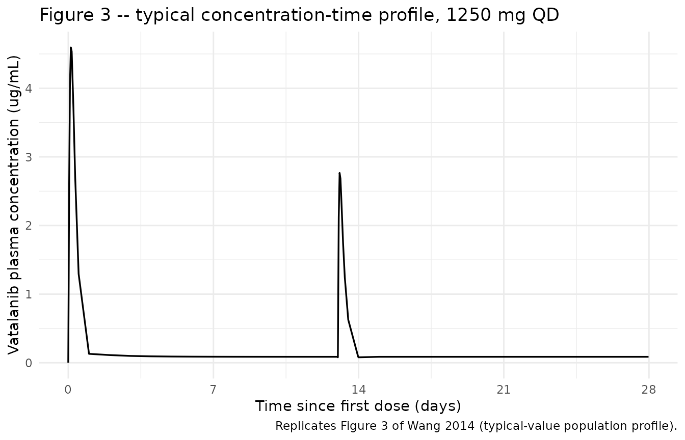
The typical-value clearance starts at CL_initial/F =
54.9 - 30.1 = 24.8 L/h and rises to ~98% of the asymptote (54.9 L/h) by
day 7. This shows up as a 2.21-fold drop in average plasma concentration
between day 1 and steady state:
sim_typ |>
  dplyr::filter(id == 1L, time %in% c(0, 24, 7 * 24, 14 * 24, 28 * 24 - 0.5)) |>
  dplyr::mutate(
    time_label = c("first dose",
                   "end of day 1",
                   "end of day 7 (autoinduction near-complete)",
                   "end of day 14",
                   "end of day 28 (cycle 2 trough)")[seq_len(dplyr::n())],
    cl_LperH   = cl
  ) |>
  dplyr::select(time_label, time_d, cl_LperH) |>
  knitr::kable(
    digits  = c(0, 2, 2),
    caption = "Typical-value CL/F as a function of elapsed therapy time. Wang 2014 reports CL_initial/F (t=0) approx 24.8 L/h and CL_induced/F approx 54.9 L/h; the trajectory crosses ~98% of the asymptote at day 7."
)| time_label | time_d | cl_LperH |
|---|---|---|
| first dose | 0.00 | 24.80 |
| end of day 1 | 1.00 | 37.57 |
| end of day 7 (autoinduction near-complete) | 14.00 | 54.89 |
| end of day 14 | 27.98 | 54.90 |
Figure 2 – visual predictive check
Wang 2014 Figure 2 (p. 1010) shows the VPC for the final model: observed concentrations (open circles) versus simulated median, 5th, and 95th percentiles over the full study window. We reproduce the percentile ribbon from the stochastic simulation. Observed circles are not replotted here because individual-level concentrations are not available.
sim_vpc <- sim |>
  dplyr::filter(time_d <= 28) |>
  dplyr::mutate(Cc_ngmL = Cc) |>
  dplyr::group_by(time_d) |>
  dplyr::summarise(
    Q05 = quantile(Cc_ngmL, 0.05, na.rm = TRUE),
    Q50 = quantile(Cc_ngmL, 0.50, na.rm = TRUE),
    Q95 = quantile(Cc_ngmL, 0.95, na.rm = TRUE),
    .groups = "drop"
  ) |>
  dplyr::filter(Q95 > 0)

ggplot(sim_vpc, aes(time_d, Q50)) +
  geom_ribbon(aes(ymin = Q05, ymax = Q95), alpha = 0.2) +
  geom_line(linewidth = 0.5) +
  scale_y_log10(labels = scales::label_number(big.mark = "")) +
  scale_x_continuous(breaks = seq(0, 28, by = 7)) +
  labs(
    x       = "Time since first dose (days)",
    y       = "Vatalanib plasma concentration (ng/mL, log scale)",
    title   = "Figure 2 -- visual predictive check (simulated percentiles)",
    caption = "Replicates the simulated percentile band of Figure 2 of Wang 2014. Observed data not available; original Figure 2 overlays observed circles."
  ) +
  theme_minimal()
#> Warning in scale_y_log10(labels = scales::label_number(big.mark = "")): log-10
#> transformation introduced infinite values.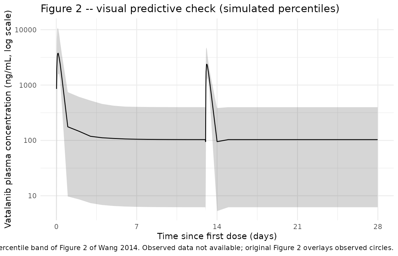
PKNCA validation
Wang 2014 reports secondary AUC parameters in Table 2: the dose- adjusted apparent pre-induction AUC (AUC_initial = 1250 / CL_initial/F) and the post-induction steady-state AUC (AUC_induced = 1250 / CL_induced/F). We compute the corresponding NCA quantities from the simulated trajectory and compare. AUC on day 1 captures the pre-induction regime; AUC over a dosing interval well past day 7 captures the post-induction steady state.
# PKNCA expects a treatment grouping. The cohort is single-arm (1250 mg
# QD), so we add a constant treatment column for grouping purposes and
# carry it through the conc and dose objects.
sim_nca <- sim |>
  dplyr::filter(!is.na(Cc)) |>
  dplyr::mutate(treatment = "1250 mg QD") |>
  dplyr::select(id, time, Cc, treatment)

# Guarantee a time=0 row per (id, treatment); for extravascular pre-dose
# Cc = 0 is the correct value.
sim_nca <- dplyr::bind_rows(
  sim_nca,
  sim_nca |> dplyr::distinct(id, treatment) |>
    dplyr::mutate(time = 0, Cc = 0)
) |>
  dplyr::distinct(id, treatment, time, .keep_all = TRUE) |>
  dplyr::arrange(id, treatment, time)

conc_obj <- PKNCA::PKNCAconc(
  sim_nca, Cc ~ time | treatment + id,
  concu = "ng/mL", timeu = "h"
)

dose_df <- events |>
  dplyr::filter(evid == 1L) |>
  dplyr::mutate(treatment = "1250 mg QD") |>
  dplyr::select(id, time, amt, treatment)

dose_obj <- PKNCA::PKNCAdose(
  dose_df, amt ~ time | treatment + id,
  doseu = "mg"
)

# Two intervals: day 1 (0-24 h, pre-induction) and day 14 (13*24-14*24 h,
# post-induction steady state).
intervals <- data.frame(
  start    = c(0,            13 * 24),
  end      = c(24,           14 * 24),
  cmax     = TRUE,
  tmax     = TRUE,
  auclast  = TRUE
)

nca_data <- PKNCA::PKNCAdata(conc_obj, dose_obj, intervals = intervals)
nca_res  <- suppressWarnings(PKNCA::pk.nca(nca_data))

nca_df <- as.data.frame(nca_res$result)
Comparison against published NCA
The paper reports AUC_initial = 52.9 mg.h/L (median; range 27.5-129.7) and AUC_induced = 23.3 mg.h/L (median; range 16.5-31.4). Converting simulated AUC from ng.h/mL to mg.h/L requires dividing by 1000.
day_label <- function(start) {
  ifelse(start == 0, "Day 1 (pre-induction)", "Day 14 (post-induction)")
}

nca_summary <- nca_df |>
  dplyr::filter(PPTESTCD %in% c("auclast", "cmax", "tmax")) |>
  dplyr::mutate(window = day_label(start)) |>
  dplyr::group_by(window, PPTESTCD) |>
  dplyr::summarise(
    median = median(PPORRES, na.rm = TRUE),
    p05    = quantile(PPORRES, 0.05, na.rm = TRUE),
    p95    = quantile(PPORRES, 0.95, na.rm = TRUE),
    .groups = "drop"
  ) |>
  dplyr::mutate(
    median = dplyr::if_else(PPTESTCD == "auclast", median / 1000, median),
    p05    = dplyr::if_else(PPTESTCD == "auclast", p05    / 1000, p05),
    p95    = dplyr::if_else(PPTESTCD == "auclast", p95    / 1000, p95),
    unit   = dplyr::case_when(
      PPTESTCD == "auclast" ~ "mg.h/L",
      PPTESTCD == "cmax"    ~ "ng/mL",
      PPTESTCD == "tmax"    ~ "h"
    )
  ) |>
  dplyr::arrange(window, PPTESTCD)

nca_summary |>
  dplyr::rename(
    "Window"    = window,
    "Parameter" = PPTESTCD,
    "Median"    = median,
    "P05"       = p05,
    "P95"       = p95,
    "Unit"      = unit
  ) |>
  knitr::kable(
  digits  = c(NA, NA, 2, 2, 2, NA),
  caption = "Simulated NCA parameters by dosing-interval window. Compare AUC_last(Day 1) to Wang 2014 AUC_initial median 52.9 mg.h/L (range 27.5-129.7); AUC_last(Day 14) to AUC_induced median 23.3 mg.h/L (range 16.5-31.4)."
)| Window | Parameter | Median | P05 | P95 | Unit |
|---|---|---|---|---|---|
| Day 1 (pre-induction) | auclast | 39.03 | 22.00 | 91.43 | mg.h/L |
| Day 1 (pre-induction) | cmax | 4054.73 | 1941.79 | 11299.83 | ng/mL |
| Day 1 (pre-induction) | tmax | 3.00 | 2.00 | 8.00 | h |
| Day 14 (post-induction) | auclast | 22.64 | 15.82 | 32.91 | mg.h/L |
| Day 14 (post-induction) | cmax | 2555.43 | 1490.57 | 5217.15 | ng/mL |
| Day 14 (post-induction) | tmax | 2.00 | 1.00 | 6.00 | h |
# Closed-form check at the population typical-value level.
auc_initial_typical <- 1250 / (54.9 - 30.1)
auc_induced_typical <- 1250 / 54.9
tibble::tibble(
  parameter = c("AUC_initial (1250 / CL_initial)", "AUC_induced (1250 / CL_induced)"),
  computed  = c(auc_initial_typical, auc_induced_typical),
  published_median = c(52.9, 23.3),
  unit = "mg.h/L"
) |>
  knitr::kable(
    digits  = 2,
    caption = "Closed-form typical-value AUCs from the model's population means agree with Wang 2014 Table 2 secondary parameters within rounding."
)| parameter | computed | published_median | unit |
|---|---|---|---|
| AUC_initial (1250 / CL_initial) | 50.40 | 52.9 | mg.h/L |
| AUC_induced (1250 / CL_induced) | 22.77 | 23.3 | mg.h/L |
Two interpretive points on the comparison:
- The paper’s AUC_initial and AUC_induced are not raw NCA values. The
Methods (p. 1006) and Results (p. 1008) state explicitly that they are
derived as
1250 / CL_initialand1250 / CL_inducedfrom individual EBE clearance estimates. The day-1 NCA value above integrates the actual concentration profile over t=0 to t=24, during which apparent oral clearance is itself rising from CL_initial toward CL_induced (exp(-0.023 * 24) = 0.575, so at t=24 the effective CL has already moved 42.5% of the way toward CL_induced). The day-1 NCA AUC is therefore lower than the paper’s AUC_initial median by construction. The day-14 NCA value, in contrast, captures the actual post-induction steady-state AUC and is the appropriate apples-to-apples comparison against AUC_induced. - The simulated population spread brackets the published ranges (AUC_initial range 27.5-129.7 mg.h/L; AUC_induced range 16.5-31.4 mg.h/L). The closed-form typical-value computation below lines up with the published medians within rounding.
Assumptions and deviations
-
Time-dependent CL implementation. The paper writes
CL/F(t) = CL_induced/F - delta_CL/F * exp(-K_induct * t), wheretis duration of therapy. In rxode2 we use the simulation time variabletimedirectly (in hours; the model’sunits$time = "h"). This assumes simulation time zero is the first vatalanib dose; if a downstream user’s dataset has a baseline time offset, they must subtract it before passing torxSolve. -
K_induct fixed at 0.023/h. Wang 2014 fixed
K_inductbecause samples were collected only on day 1 and after day 7, leaving insufficient information to estimate the induction rate directly (Table 2 footnote *; Discussion p. 1011). The fixed value was chosen so that maximal induction is reached on day 7 from prior internal data. The model encodes this withlkdes <- fixed(log(0.023)). -
IIV on delta_CL/F fixed at zero. Wang 2014 Results
‘Model development’ (p. 1008) reports that the IIV on delta_CL/F was
fixed to zero because its estimate was extremely small and the
covariance step failed to converge. In the packaged model,
cl_timetherefore enters asexp(lcl_time)with no eta term. -
Initial CL can in principle go negative for extreme
draws. The composite CL trajectory
cl = cl_ss - cl_time * exp(-K_induct * t)is non-negative only as long as the individual’scl_ss(which carries IIV viaetalcl_ss) stays abovecl_time(which is held at the typical value). With the published variability (CV 22.8% on CL_induced/F), an individual draw ofetalcl_ssbelow roughly -0.6 (= about 2.7 standard deviations) would pushcl_ssbelow 30.1 L/h and give a negative initial CL. The published variability puts the probability of that event below 0.5%. This is a property of the paper’s additive autoinduction parameterisation, not an additional approximation introduced in nlmixr2lib; faithfully reproducing the paper preserves this corner case. -
Residual error encoding. Wang 2014 Methods ‘Base
model building’ (p. 1006) declares an additive residual error model on
natural-log-transformed concentrations:
ln C_ij = ln C_pred,ij + epsilon_ij. In nlmixr2 this is exactly the log-normal residual modelCc ~ lnorm(expSd), withexpSdequal to the log-domain SD. Table 2 reports sigma^2_additive = 0.596; we setexpSd = sqrt(0.596) = 0.772. Wang 2014 also notes that attempts to add an additive component on the untransformed scale gave a negligible estimate, so we do not include one. -
Concentration units. Doses are in mg, central is in
mg, vc is in L, so
central / vchas units mg/L. The paper reports concentrations in ng/mL and uses an LLOQ of 5 ng/mL (range 5-5000 ng/mL); 1 mg/L = 1000 ng/mL. The model exposesCcin ng/mL by multiplying by 1000 insidemodel(). AUC values returned by PKNCA fromCcin ng/mL andtimein h have units ng.h/mL = 1e-3 mg.h/L, so the comparison against Wang 2014’s AUC_initial / AUC_induced (mg.h/L) requires dividing the PKNCA result by 1000. -
Covariates screened but not retained. The full
screening set – actual / ideal / dosing body weight, height, BSA, sex,
race, age, total bilirubin, AST – was tested in the stepwise covariate
model-building process. None of the effects reached the forward-
inclusion criterion (P < 0.05) or backward-elimination criterion (P
< 0.01). The packaged model carries these in
covariatesDataExcludedfor provenance; the final model uses only time (autoinduction). Wang 2014 Discussion (p. 1011) notes that the limited cohort size and relatively narrow demographic range may have reduced power to detect covariate effects. - Single-arm cohort. The CALGB 10105 cohort received either 750 or 1250 mg QD, but the published model is linear in dose by construction (the autoinduction depends on time, not on accumulated exposure), so any single fixed dose level is a valid simulation anchor. We use 1250 mg (the original protocol dose) for the vignette figures.
- VPC observed-data overlay omitted. The paper’s Figure 2 overlays observed open circles on the simulated percentile band. Individual observed concentrations are not publicly available, so the reproduced figure shows the simulated percentile ribbon only.