Voriconazole plasma and saliva (Kim 2020)
Source:vignettes/articles/Kim_2020_voriconazole.Rmd
Kim_2020_voriconazole.RmdModel and source
- Citation: Kim HY, Martson A-G, Dreesen E, Spriet I, Wicha SG, McLachlan AJ, Alffenaar J-W. Saliva for Precision Dosing of Antifungal Drugs: Saliva Population PK Model for Voriconazole Based on a Systematic Review. Front Pharmacol. 2020;11:894. doi:10.3389/fphar.2020.00894
- Description: One-compartment population PK model for oral and intravenous voriconazole in hospitalised patients treated for invasive aspergillosis (Kim 2020), fitted jointly to paired plasma and saliva concentrations. Oral doses enter a gut depot with bioavailability 0.849 and first-order absorption (ka fixed at 0.858 1/h); intravenous doses enter the central (plasma) compartment directly. Saliva is not a separate kinetic compartment: the salivary voriconazole concentration is the plasma concentration multiplied by an estimated saliva:plasma scale factor of 0.501, a structure the authors selected over a separate saliva compartment (dOFV = -102.7). IIV on clearance only; no covariates; separate proportional residual errors for plasma and saliva.
- Article: https://doi.org/10.3389/fphar.2020.00894
Kim and colleagues first systematically reviewed the evidence for saliva-based therapeutic drug monitoring (TDM) of antifungal drugs, and then – for the drug with the strongest evidence, voriconazole – built a population PK model that describes plasma and saliva concentrations simultaneously. The systematic-review half of the paper tabulates published saliva/plasma (S/P) ratios but contains no model; only the population PK model is packaged here.
The final structure (Figure 2 of the paper) is a one-compartment
model with first-order absorption. Oral doses pass through a gut depot
with bioavailability F; intravenous doses enter plasma
directly. Saliva is not given its own compartment: its concentration is
the plasma concentration multiplied by an estimated scale factor, which
fit better (dOFV -102.7) than a separate saliva compartment. The
packaged model therefore has two ODE states (depot,
central) and two observations, Cc (plasma) and
Csaliva = fsaliva * Cc.
Population
Individual data were obtained from one of the reviewed studies (Vanstraelen et al. 2015): 11 patients (10 adults and one 9-year-old child) treated with voriconazole for invasive aspergillosis on oncology/haematology (8) or respiratory (3) wards, or a paediatric ward. Seven were male and four female. Adult median age was 55 years (range 30-66) and adult mean body weight 65.9 +/- 20.1 kg (Kim 2020 Results, “Data Retrieval From Authors’ Studies”). Patients received voriconazole intravenously or orally every 12 h for at least 4 days (3.7 +/- 0.4 mg/kg, Table 2), and paired plasma and saliva samples were drawn at steady state at pre-dose, 0.5, 1, 1.5, 2, 6 and 12 h after the dose: 69 plasma and 68 saliva concentrations in total.
The same information is available programmatically via
readModelDb("Kim_2020_voriconazole")()$population.
Source trace
| Equation / parameter | Value | Source location |
|---|---|---|
lcl (theta_1) |
4.56 L/h | Table 4 (RSE 16%; bootstrap 4.39 [3.23-5.98]) |
lvc (theta_2) |
60.7 L | Table 4 (RSE 12%; bootstrap 57.9 [41.4-72.3]) |
lka (theta_3) |
0.858 1/h, fixed | Table 4 “fixed to model estimate”; Results (RSE 129% when estimated) |
lfdepot (theta_4) |
0.849 | Table 4 (RSE 14%; bootstrap 0.819 [0.577-0.983]) |
lfsaliva (theta_5) |
0.501 | Table 4 (RSE 4%; bootstrap 0.499 [0.458-0.541]) |
etalcl |
0.136 | Table 4 omega^2 on CL (36.9% CV) |
propSd |
sqrt(0.057) = 0.239 | Table 4 sigma^2 proportional, plasma = 0.057 |
propSd_Csaliva |
sqrt(0.078) = 0.279 | Table 4 sigma^2 proportional, saliva = 0.078 |
d/dt(depot) = -ka * depot;
f(depot) = F
|
n/a | Figure 2 (oral dose -> F -> gut -> ka -> plasma) |
d/dt(central) = ka * depot - CL/V * central |
n/a | Figure 2; Results (one-compartment, first-order absorption and elimination; ADVAN13) |
IV dose into central
|
n/a | Figure 2 (IV dose -> plasma) |
Csaliva = fsaliva * Cc |
n/a | Figure 2 (scale factor from plasma to saliva); Results |
| Proportional error on each matrix | n/a | Results, “Salivary Pharmacokinetics of Voriconazole” |
Table 4 reports variances (omega^2, sigma^2). The CL IIV is encoded
directly as the log-scale variance 0.136; the paper’s “36.9% CV” is
sqrt(0.136). The residual SDs are the square roots of the
sigma^2 values.
Virtual cohort
The observed data are not public. The virtual cohort follows the
study design: voriconazole 3.7 mg/kg every 12 h, either orally or as an
intravenous infusion, in adults whose body weight is drawn from a normal
distribution with the reported mean and SD (65.9 +/- 20.1 kg), truncated
to 40-120 kg. Body weight is not a model covariate; it only sets each
subject’s mg/kg dose. Dosing runs for 7 days (14 doses) so that the last
interval (156-168 h) is at steady state (the typical half-life is
log(2) * 60.7 / 4.56 = 9.2 h). Two arms of 200
subjects:
-
Oral q12h – dose into
depot. -
IV q12h – 2-h infusion into
central.
set.seed(20200612)
rxode2::rxSetSeed(20200612)

n_per_arm <- 200L
dose_mgkg <- 3.7
tau <- 12
dose_times <- seq(0, by = tau, length.out = 14)   # last dose at 156 h
t_last <- max(dose_times)
obs_times <- t_last + c(0, 0.25, 0.5, 0.75, 1, 1.25, 1.5, 1.75, 2, 2.5, 3, 4,
                        5, 6, 7, 8, 9, 10, 11, 12)

rtrunc_norm <- function(n, mean, sd, lower, upper) {
  out <- rnorm(n, mean, sd)
  bad <- out < lower | out > upper
  while (any(bad)) {
    out[bad] <- rnorm(sum(bad), mean, sd)
    bad <- out < lower | out > upper
  }
  out
}

make_arm <- function(treatment, dose_cmt, dur, id_offset) {
  subj <- tibble(
    id = id_offset + seq_len(n_per_arm),
    treatment = treatment,
    WT = rtrunc_norm(n_per_arm, 65.9, 20.1, 40, 120)
  ) |>
    mutate(dose_mg = dose_mgkg * WT)
  doses <- subj |>
    tidyr::crossing(time = dose_times) |>
    mutate(evid = 1L, amt = dose_mg, dur = dur, cmt = dose_cmt, dvid = NA_integer_)
  obs <- subj |>
    tidyr::crossing(time = obs_times, dvid = c(1L, 2L)) |>
    mutate(evid = 0L, amt = NA_real_, dur = NA_real_, cmt = "central")
  bind_rows(doses, obs)
}

events <- bind_rows(
  make_arm("Oral q12h", "depot", NA_real_, id_offset = 0L),
  make_arm("IV q12h", "central", 2, id_offset = n_per_arm)
) |>
  arrange(id, time, desc(evid))

stopifnot(dplyr::n_distinct(events$id) == 2L * n_per_arm)
Simulation
dvid = 1 rows return the plasma observation and
dvid = 2 rows the saliva observation in sim,
each with its own proportional residual error; Cc and
Csaliva are the residual-free individual predictions on
every row.
mod <- readModelDb("Kim_2020_voriconazole")

sim <- as.data.frame(rxode2::rxSolve(
  mod, events = events,
  keep = c("treatment", "WT", "dose_mg", "dvid"),
  maxsteps = 1e6
)) |>
  mutate(
    matrix = ifelse(dvid == 1L, "Plasma", "Saliva"),
    conc_obs = sim,
    conc_ipred = ifelse(dvid == 1L, Cc, Csaliva),
    tad = time - t_last
  )
#> ℹ parameter labels from comments will be replaced by 'label()'

stopifnot(
  dplyr::n_distinct(sim$id) == 2L * n_per_arm,
  all(is.finite(sim$conc_ipred))
)
A typical-value solve (no IIV, no residual error) feeds the structural checks.
typ_events <- bind_rows(
  tibble(id = 1L, treatment = "Oral q12h", cmt = "depot", dur = NA_real_),
  tibble(id = 2L, treatment = "IV q12h", cmt = "central", dur = 2)
) |>
  mutate(dose_mg = dose_mgkg * 65.9)

typ_ev <- bind_rows(
  typ_events |>
    tidyr::crossing(time = dose_times) |>
    mutate(evid = 1L, amt = dose_mg, dvid = NA_integer_),
  typ_events |>
    select(-cmt, -dur) |>
    tidyr::crossing(time = t_last + seq(0, 12, by = 0.05), dvid = c(1L, 2L)) |>
    mutate(evid = 0L, amt = NA_real_, dur = NA_real_, cmt = "central")
) |>
  arrange(id, time, desc(evid))

typ <- as.data.frame(rxode2::rxSolve(
  rxode2::zeroRe(mod), events = typ_ev,
  keep = c("treatment", "dose_mg", "dvid"), omega = NA,
  rtol = 1e-10, atol = 1e-12, maxsteps = 1e6
)) |>
  mutate(tad = time - t_last)
#> ℹ parameter labels from comments will be replaced by 'label()'
#> Warning: multi-subject simulation without without 'omega'

stopifnot(isTRUE(all.equal(unique(typ$cl), 4.56, tolerance = 1e-8)))
Replicate published figures
Figure 7: visual predictive check by matrix
Figure 7 of Kim 2020 is the prediction-corrected VPC of plasma (A) and saliva (B) concentrations against time after dose over a steady-state dosing interval. The simulated 5th / 50th / 95th percentiles of the observations are shown per matrix and route. The paper’s observed concentrations span roughly 0.5-10 mg/L in plasma and about half that in saliva.
sim |>
  group_by(treatment, matrix, tad) |>
  summarise(
    Q05 = quantile(conc_obs, 0.05, na.rm = TRUE),
    Q50 = quantile(conc_obs, 0.50, na.rm = TRUE),
    Q95 = quantile(conc_obs, 0.95, na.rm = TRUE),
    .groups = "drop"
  ) |>
  ggplot(aes(tad, Q50, colour = treatment, fill = treatment)) +
  geom_ribbon(aes(ymin = Q05, ymax = Q95), alpha = 0.2, colour = NA) +
  geom_line(linewidth = 0.8) +
  facet_wrap(~matrix) +
  labs(
    x = "Time after dose (h)", y = "Voriconazole concentration (mg/L)",
    colour = NULL, fill = NULL,
    title = "Simulated 5th / 50th / 95th percentiles at steady state",
    caption = "Replicates Figure 7 (A: plasma, B: saliva) of Kim 2020."
  )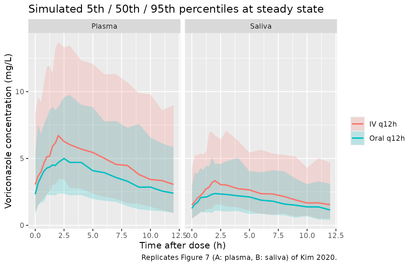
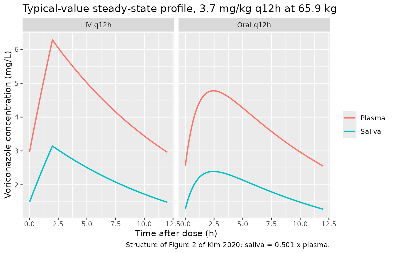
Figure 2: the saliva/plasma ratio is the scale factor at every time
Because saliva is the plasma compartment rescaled, the
individual-prediction S/P ratio equals fsaliva = 0.501 at
every time for every subject – the “identical kinetics, lower extent”
finding stated in the Discussion.
ratio_ipred <- sim |>
  filter(Cc > 1e-9) |>
  mutate(ratio = Csaliva / Cc) |>
  pull(ratio)
stopifnot(isTRUE(all.equal(range(ratio_ipred), c(0.501, 0.501), tolerance = 1e-8)))

typ |>
  filter(dvid == 1L) |>
  select(treatment, tad, Plasma = Cc, Saliva = Csaliva) |>
  tidyr::pivot_longer(c(Plasma, Saliva), names_to = "matrix", values_to = "conc") |>
  ggplot(aes(tad, conc, colour = matrix)) +
  geom_line(linewidth = 0.8) +
  facet_wrap(~treatment) +
  labs(
    x = "Time after dose (h)", y = "Voriconazole concentration (mg/L)", colour = NULL,
    title = "Typical-value steady-state profile, 3.7 mg/kg q12h at 65.9 kg",
    caption = "Structure of Figure 2 of Kim 2020: saliva = 0.501 x plasma."
  )
Closed-form steady-state AUC
For a linear one-compartment model the AUC over a steady-state dosing
interval equals F * Dose / CL (oral) or
Dose / CL (IV), times 0.501 for saliva. This checks the
dose route, bioavailability placement and units of the model.
auc_typ <- typ |>
  filter(dvid == 1L) |>
  group_by(treatment) |>
  summarise(
    auc_plasma = sum(diff(tad) * (head(Cc, -1) + tail(Cc, -1)) / 2),
    auc_saliva = sum(diff(tad) * (head(Csaliva, -1) + tail(Csaliva, -1)) / 2),
    dose_mg = first(dose_mg),
    .groups = "drop"
  ) |>
  mutate(
    f = ifelse(treatment == "Oral q12h", 0.849, 1),
    auc_closed = f * dose_mg / 4.56,
    pct_plasma = 100 * (auc_plasma / auc_closed - 1),
    pct_saliva = 100 * (auc_saliva / (0.501 * auc_closed) - 1)
  )

auc_typ |>
  transmute(
    Arm = treatment,
    `Plasma AUCtau, integrated (mg*h/L)` = round(auc_plasma, 2),
    `Plasma AUCtau = F*Dose/CL (mg*h/L)` = round(auc_closed, 2),
    `Saliva AUCtau, integrated (mg*h/L)` = round(auc_saliva, 2),
    `Saliva AUCtau = 0.501*F*Dose/CL (mg*h/L)` = round(0.501 * auc_closed, 2)
  ) |>
knitr::kable(caption = "Typical-value steady-state AUC over one 12-h interval.")| Arm | Plasma AUCtau, integrated (mg*h/L) | Plasma AUCtau = FDose/CL (mgh/L) | Saliva AUCtau, integrated (mg*h/L) | Saliva AUCtau = 0.501FDose/CL (mg*h/L) |
|---|---|---|---|---|
| IV q12h | 53.47 | 53.47 | 26.79 | 26.79 |
| Oral q12h | 45.40 | 45.40 | 22.74 | 22.74 |
PKNCA validation
NCA over the steady-state interval (156-168 h), per matrix, with the
dosing route as the treatment grouping. NCA is run on the individual
predictions (Cc, Csaliva) rather than on the
residual-error observations: with proportional residual SDs of
0.24-0.28, an occasional simulated observation is negative, which PKNCA
cannot integrate, and residual noise would only bias the grid maximum
upward.
nca_dose <- events |>
  filter(evid == 1L, time == t_last) |>
  select(id, time, amt, treatment)

run_nca <- function(matrix_name) {
  conc <- sim[sim$matrix == matrix_name, ] |>
    filter(!is.na(conc_ipred)) |>
    select(id, time, treatment, Cc = conc_ipred)
  conc_obj <- PKNCA::PKNCAconc(conc, Cc ~ time | treatment + id)
  dose_obj <- PKNCA::PKNCAdose(nca_dose, amt ~ time | treatment + id)
  intervals <- data.frame(
    start = t_last, end = t_last + tau,
    cmax = TRUE, tmax = TRUE, cmin = TRUE, auclast = TRUE
  )
  res <- PKNCA::pk.nca(PKNCA::PKNCAdata(conc_obj, dose_obj, intervals = intervals))
  as.data.frame(res) |>
    mutate(matrix = matrix_name)
}

nca <- bind_rows(run_nca("Plasma"), run_nca("Saliva"))
Comparison against the source study
Kim 2020 does not report NCA for its own model, but Table 2 of the
paper summarises the source study’s (Vanstraelen 2015) observed
steady-state exposure in these patients as median (IQR): plasma (total)
Cmax 6.0 (4.0-9.3) mg/L and AUC0-12 47.0 (28.7-66.6) mgh/L; saliva
Cmax 3.3 (2.7-4.2) mg/L and AUC0-12 23.9 (15.8-32.1) mgh/L. Those
values pool oral and IV patients, so the same reference row is set
against each simulated route. A pooled oral/IV median should fall
between the two simulated routes, which differ in AUC by the factor
1/F = 1.18. It does: the oral arm’s AUC0-12 is about 5%
below and the IV arm’s about 18-20% above the observed medians in both
matrices. The observed Cmax medians likewise fall between the oral and
IV arms; the oral Cmax sits 19-26% below them, partly because the
observed Cmax is the maximum of noisy measured samples while the
simulated one is taken from residual-free predictions.
ref_one <- tibble::tribble(
  ~matrix,  ~cmax, ~auclast,
  "Plasma", 6.0,   47.0,
  "Saliva", 3.3,   23.9
)
published_nca <- bind_rows(
  mutate(ref_one, treatment = "Oral q12h"),
  mutate(ref_one, treatment = "IV q12h")
)

cmp <- nlmixr2lib::ncaComparisonTable(
  simulated = nca |> filter(PPTESTCD %in% c("cmax", "auclast")),
  reference = published_nca,
  by = c("treatment", "matrix"),
  units = c(cmax = "mg/L", auclast = "mg*h/L"),
  tolerance_pct = 20
)

knitr::kable(
  cmp,
  caption = "Simulated steady-state NCA vs. observed medians (Kim 2020 Table 2, Vanstraelen 2015 row). * differs by >20%.",
  align = c("l", "l", "l", "r", "r", "r")
)| NCA parameter | treatment | matrix | Reference | Simulated | % diff |
|---|---|---|---|---|---|
| Cmax (mg/L) | Oral q12h | Plasma | 6 | 4.87 | -18.8% |
| Cmax (mg/L) | Oral q12h | Saliva | 3.3 | 2.44 | -26.0%* |
| Cmax (mg/L) | IV q12h | Plasma | 6 | 6.7 | +11.6% |
| Cmax (mg/L) | IV q12h | Saliva | 3.3 | 3.35 | +1.7% |
| AUClast (mg*h/L) | Oral q12h | Plasma | 47 | 44.8 | -4.6% |
| AUClast (mg*h/L) | Oral q12h | Saliva | 23.9 | 22.5 | -6.0% |
| AUClast (mg*h/L) | IV q12h | Plasma | 47 | 56.2 | +19.6% |
| AUClast (mg*h/L) | IV q12h | Saliva | 23.9 | 28.2 | +17.8% |
attr(cmp, "footnote")
#> [1] "* differs from reference by more than ±20%."

auc_med <- nca |>
  filter(PPTESTCD == "auclast") |>
  group_by(treatment, matrix) |>
  summarise(med = median(PPORRES), .groups = "drop")

# Structural: the simulated median AUCtau of each route sits inside the observed
# IQR of the pooled oral/IV population (plasma 28.7-66.6, saliva 15.8-32.1).
stopifnot(
  all(auc_med$med[auc_med$matrix == "Plasma"] > 28.7 &
        auc_med$med[auc_med$matrix == "Plasma"] < 66.6),
  all(auc_med$med[auc_med$matrix == "Saliva"] > 15.8 &
        auc_med$med[auc_med$matrix == "Saliva"] < 32.1)
)
Saliva/plasma ratio
The observed S/P ratio in the source study was 0.51 +/- 0.08 (total drug; Table 2), and the review-wide average across the four voriconazole studies was 0.56 +/- 0.18 (Results). With residual error on both matrices the simulated per-sample S/P ratio scatters around the scale factor 0.501.
sp <- sim |>
  select(id, time, treatment, matrix, conc_obs) |>
  tidyr::pivot_wider(names_from = matrix, values_from = conc_obs) |>
  mutate(sp = Saliva / Plasma)

sp_auc <- nca |>
  filter(PPTESTCD == "auclast") |>
  select(id, treatment, matrix, PPORRES) |>
  tidyr::pivot_wider(names_from = matrix, values_from = PPORRES) |>
  mutate(sp = Saliva / Plasma)

tibble(
  Quantity = c("Per-sample S/P ratio", "AUC0-12 S/P ratio"),
  `Simulated median` = round(c(median(sp$sp), median(sp_auc$sp)), 3),
  `Observed (Vanstraelen 2015, Table 2)` = c("0.51 +/- 0.08", "23.9 / 47.0 = 0.51")
) |>
knitr::kable(caption = "Saliva/plasma ratio: simulated vs. observed.")| Quantity | Simulated median | Observed (Vanstraelen 2015, Table 2) |
|---|---|---|
| Per-sample S/P ratio | 0.498 | 0.51 +/- 0.08 |
| AUC0-12 S/P ratio | 0.501 | 23.9 / 47.0 = 0.51 |
Assumptions and deviations
- Dosing. 3.7 mg/kg every 12 h is the source study’s mean dose (Table 2). Individual doses, routes and the oral/IV split are not reported, so both routes are simulated separately. The intravenous infusion duration is not reported; 2 h is assumed (within the usual 1-2 h voriconazole infusion). The infusion duration affects the IV Cmax but not AUC.
- Body weight. Drawn from a normal distribution with the reported adult mean and SD (65.9 +/- 20.1 kg), truncated to 40-120 kg. Weight is not a model covariate (weight, AST, ALT, ALP and bilirubin on CL were tested and rejected, Results) and only scales the mg/kg dose. The single paediatric patient in the analysis dataset is not represented in the virtual cohort.
-
Bioavailability on the oral route only. Figure 2
places
Fbetween the oral dose and the gut; intravenous doses enter plasma directly, sof(depot)is the only bioavailability term. - Scale factor has no IIV. The paper did not estimate IIV on the scale factor (the Discussion names this as a limitation of the small dataset), so all saliva/plasma variability in the model is residual.
- Comparison references pool routes. The Table 2 exposure medians come from the source study’s mixed oral and intravenous population and are compared with each simulated route separately. As expected for a pooled reference, the observed medians fall between the oral and IV arms (see the comparison table), and the starred oral saliva Cmax row reflects the route split and the residual-free simulated Cmax rather than a structural mismatch. The IV Cmax also depends on the assumed 2-h infusion.
- Systematic review not packaged. The paper’s systematic review (Tables 1-3) summarises published S/P ratios for fluconazole, voriconazole, itraconazole and ketoconazole without any model; only the voriconazole population PK model is packaged.
- Supplement / errata. The article has no supplementary material, and no erratum was found (Europe PMC search, 2026-09-26).
-
Naming. The saliva scale factor is
lfsaliva/fsalivaand the saliva observationCsaliva, matching the identical plasma-scale-factor structure inXu_2023_busulfan.