In vivo CAR-T via CAR mRNA nanoparticle (Kim 2024)
Source:vignettes/articles/Kim_2024_car_mrna_nanoparticle.Rmd
Kim_2024_car_mrna_nanoparticle.RmdModel and source
Kim, Mugundu and Singh (2024) built a mechanism-based, cell-level PK-PD model describing the transient surface chimeric antigen receptor (CAR) expression on T cells after they are transfected with a CD8-targeted polymeric nanoparticle (NP) carrying in-vitro-transcribed 1928z CAR mRNA. The paper develops the model in two linked settings, extracted here as two model files:
Kim_2024_carmrna_invitro_qsp- the in vitro cell-level model (human CD8+ T cells in culture; Appendix S1 Eqs. 2-5).Kim_2024_carmrna_mouse_qsp- the in vivo model (immunodeficient NSG mice), which prepends a fixed two-compartment nanoparticle disposition to the same cell-level cascade (Appendix S1 Eqs. 13-17; simulation code in Appendix S2).Article: Clin Transl Sci 17(12):e70101
mv_invitro <- readModelDb("Kim_2024_carmrna_invitro_qsp")
mv_mouse <- readModelDb("Kim_2024_carmrna_mouse_qsp")
Both models share the same biology: an anti-CD8 antibody on the NP
binds a constant pool of free CD8 receptors (kon,
koff); the NP-receptor complex is internalised
(kint) and dilutes with untransduced T-cell proliferation
(kg_cell); the internalised NP releases free intracellular
mRNA that degrades (kdeg_trans); and the free mRNA drives
surface CAR protein formation through a sigmoidal Emax (Hill) process
opposed by first-order protein degradation (kdeg). All
concentration states are in pM; the readout carexpr is
percent surface CAR expression.
Population
The in vitro data come from transfecting 1e6 CD8+ T cells/mL (assumed media volume 100 uL) with 3 ug of 1928z CAR mRNA in the CD8-targeted NP, assayed at days 1, 2, 5, 8 and 10 across nine replicates. The in vivo system is immunodeficient NSG mice inoculated with 1e6 CD19+ Raji cells (firefly luciferase), reconstituted 5 days later with 1e7 CD3+ human T cells, and dosed 2 days after reconstitution with six weekly IV infusions of 50 ug of mRNA in the NP. Both time courses were digitised by the original authors from the study they cite as reference 23 (Parayath et al.); the reported in vivo mean was 10.7 +/- 3.6 percent CAR+ among CD8+ T cells.
mv_mouse()$population$dose_range
#> [1] "Six weekly IV infusions of a CD8-targeted nanoparticle loaded with 50 ug of 1928z CAR mRNA, starting 2 days after T-cell reconstitution. 50 ug / MW 1e6 Da in the fitted NP central volume V1 = 7.87 mL = 6353 pM, the per-dose mRNA_central increment."
Source trace
The per-parameter origin is recorded as an in-file comment next to
each ini() entry. The tables below collect the final
estimates (Kim 2024 Table 2) in one place.
In vitro model (Kim_2024_carmrna_invitro_qsp)
| Parameter | Value | IIV (CV%) | Source |
|---|---|---|---|
kon |
0.00202 1/pM/h | fixed | Table 2, ref 44 |
koff |
3.60 1/h | fixed | Table 2, ref 44 |
kint |
0.0133 1/h | fixed | Table 2, ref 43 |
kg_cell |
0.0134 1/h | fixed | Table 2, ref 45 |
rtot |
2483 pM | fixed | Table 2, ref 46 |
emax |
1 | fixed | Table 2 |
kdeg_trans |
0.037 1/h | fixed (30% in mRNA submodel) | Table 2 / App. S1 Eq. 6 |
ec50 |
941 pM | 3.85 | Table 2 |
hill (n1) |
13.09 | 20.28 | Table 2 |
kdeg |
1.45 1/h | 1.36 | Table 2 |
addSd (a) |
0.041 | - | Table 2 |
propSd (b) |
0.18 | - | Table 2 |
In vivo model (Kim_2024_carmrna_mouse_qsp)
| Parameter | Value | IIV (CV%) | Source |
|---|---|---|---|
knp (k) |
0.086 1/h | fixed | Table 2 |
k12 |
0.64 1/h | fixed | Table 2 |
k21 |
0.61 1/h | fixed | Table 2 |
kon |
0.00202 1/pM/h | fixed | Table 2, ref 44 |
koff |
3.60 1/h | fixed | Table 2, ref 44 |
kint |
0.0133 1/h | fixed | Table 2, ref 43 |
kg_cell |
0.0134 1/h | fixed | Table 2, ref 45 |
rtot |
2483 pM | fixed | Table 2, ref 46 |
emax |
1 | fixed | Table 2 |
kdeg_trans |
0.037 1/h | fixed | Table 2 |
ec50 |
124 pM | 12.7 | Table 2 |
hill (n1) |
1.71 | 8.25 | Table 2 |
kdeg |
0.078 1/h | 3.40 | Table 2 |
propSd (b) |
0.395 | - | Table 2 |
The fitted NP central volume V1 = 7.87 mL (RSE 2.07%)
does not appear in the ODEs (the states are concentrations); it enters
only when converting the dose mass to the central concentration below,
and in deriving rtot.
ODE systems and units
In vitro (Appendix S1 Eqs. 2-5), states in pM except
carexpr (percent):
d/dt(mrna_media) = -kon*mrna_media*rtot + koff*rc_complex
d/dt(rc_complex) =  kon*mrna_media*rtot - koff*rc_complex - kint*rc_complex - kg_cell*rc_complex
d/dt(mrna_free)  =  kint*rc_complex - kdeg_trans*mrna_free
d/dt(carexpr)    =  emax*mrna_free^hill/(ec50^hill + mrna_free^hill) - kdeg*carexpr
In vivo adds the two-compartment NP disposition (Eqs. 13-17):
d/dt(mrna_central)    = -knp*mrna_central - k12*mrna_central + k21*mrna_peripheral
                        - kon*mrna_central*rtot + koff*rc_complex
d/dt(mrna_peripheral) =  k12*mrna_central - k21*mrna_peripheral
Every term is a concentration rate (pM/h): a rate constant (1/h)
times a pM state, or kon (1/pM/h) times mrna_*
(pM) times rtot (pM). The Hill production term is
dimensionless (pM^n / pM^n) times emax, giving percent/h
after subtracting kdeg*carexpr.
Dose conversion
The model doses in pM. The paper’s mass doses convert with the assumed mRNA molecular weight of 1e6 Da and the relevant volume.
mw <- 1e6 # Da (Appendix S1)
# in vitro: 3 ug in 100 uL
dose_invitro_pM <- (3e-6 / mw) / (100e-6) * 1e12
# in vivo: 50 ug in the fitted NP central volume V1 = 7.87 mL
V1_mL <- 7.87
dose_invivo_pM <- (50e-6 / mw) / (V1_mL * 1e-3) * 1e12
c(invitro_pM = dose_invitro_pM, invivo_pM = dose_invivo_pM)
#> invitro_pM  invivo_pM
#>   30000.00    6353.24
These reproduce the paper’s initial conditions:
mrna_media(0) = 30000 pM in vitro, and a 6353 pM central
increment per 50 ug dose in vivo.
In vitro model (replicates Figure 2a)
A single transfection is a bolus into mrna_media.
Simulations are typical-value (random effects zeroed), matching the
fitted-profile figure.
m_iv <- zeroRe(rxode2(mv_invitro))
#> ℹ parameter labels from comments will be replaced by 'label()'
ev_iv <- et(amt = dose_invitro_pM, cmt = "mrna_media", time = 0) |>
  et(seq(0, 10 * 24, by = 1))
s_iv <- rxSolve(m_iv, ev_iv, returnType = "data.frame")
#> ℹ omega/sigma items treated as zero: 'etalec50', 'etalhill', 'etalkdeg'

ggplot(s_iv, aes(time / 24, carexpr)) +
  geom_line(linewidth = 0.8, colour = "#2c7fb8") +
  labs(
    x = "Time (days)", y = "Surface CAR expression (%)",
    title = "In vitro transient CAR expression after a single transfection",
    caption = "Replicates Figure 2a of Kim 2024 (typical-value profile)."
  )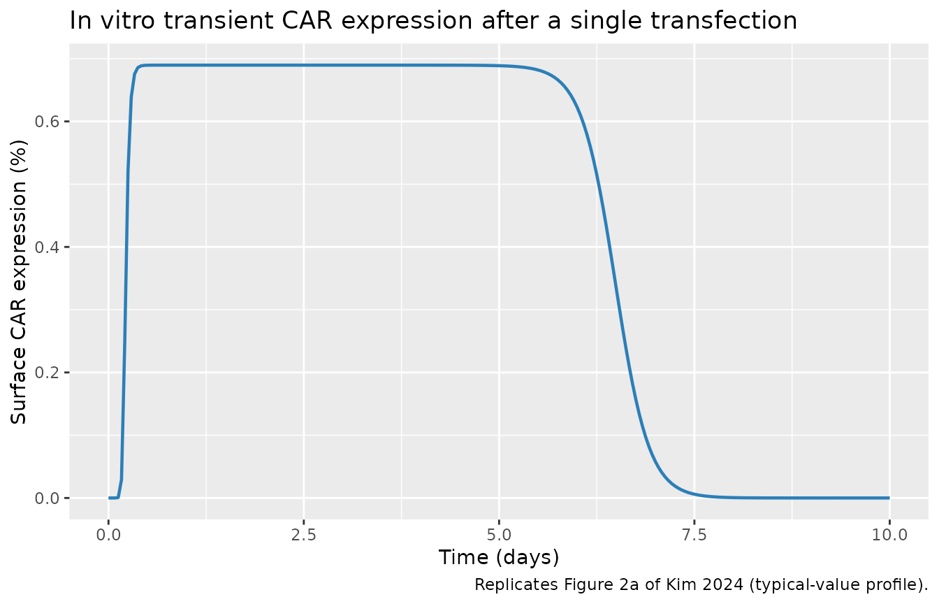
The transient peaks near day 1.7 and resolves by about day 8-10, the
window the in vitro assay sampled. The absolute magnitude is low
(sub-1%) because the in vitro protein degradation rate kdeg
= 1.45 1/h (a ~0.5 h protein half-life) is roughly 19-fold faster than
the in vivo value; the steady ceiling of the direct-effect model is
emax / kdeg.
peak_iv <- max(s_iv$carexpr)
t_peak_iv <- s_iv$time[which.max(s_iv$carexpr)] / 24
stopifnot(
  # Transient: starts and ends essentially at zero, with an interior peak.
  s_iv$carexpr[1] == 0,
  peak_iv > 0,
  s_iv$carexpr[nrow(s_iv)] < 0.5 * peak_iv,
  # Peak occurs within the first few days (the assayed window).
  t_peak_iv > 0.5, t_peak_iv < 4,
  # Direct-effect ceiling emax/kdeg = 1/1.45 ~ 0.69.
  peak_iv < 1 / 1.45 + 1e-6
)
c(peak_percent = peak_iv, t_peak_days = t_peak_iv)
#> peak_percent  t_peak_days
#>    0.6896551    1.7083333
In vivo model (replicates Figure 2b)
The original regimen is six weekly 50 ug doses. CAR expression is measured 2 days after each dose.
m_mo <- zeroRe(rxode2(mv_mouse))
#> ℹ parameter labels from comments will be replaced by 'label()'
week <- 168 # h
ev_mo <- et(amt = dose_invivo_pM, cmt = "mrna_central", time = seq(0, 5 * week, by = week)) |>
  et(seq(0, 7 * week, by = 1))
s_mo <- rxSolve(m_mo, ev_mo, returnType = "data.frame")
#> ℹ omega/sigma items treated as zero: 'etalec50', 'etalhill', 'etalkdeg'

ggplot(s_mo, aes(time / 24, carexpr)) +
  geom_line(linewidth = 0.8, colour = "#2c7fb8") +
  geom_hline(yintercept = 10.7, linetype = "dashed", colour = "grey40") +
  annotate("rect",
    xmin = -Inf, xmax = Inf, ymin = 10.7 - 3.6, ymax = 10.7 + 3.6,
    alpha = 0.12, fill = "grey40"
  ) +
  labs(
    x = "Time (days)", y = "Surface CAR expression on CD8+ T cells (%)",
    title = "In vivo transient CAR expression, six weekly 50 ug doses",
    caption = "Replicates Figure 2b of Kim 2024; band is the observed 10.7 +/- 3.6%."
  )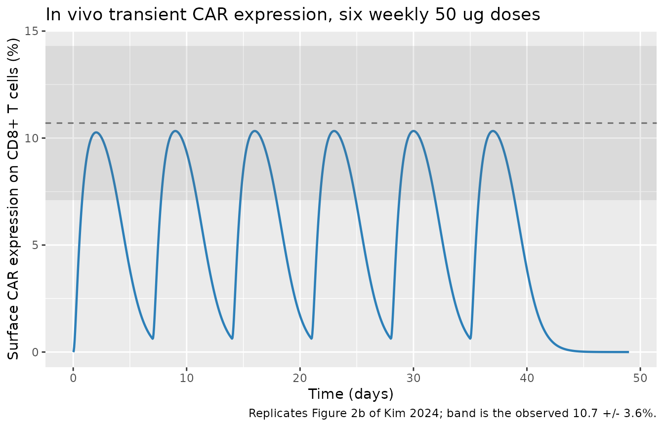
The published mean among CD8+ T cells was 10.7 +/- 3.6 percent CAR+. The model’s CAR expression measured 2 days after each dose sits squarely in that band, and expression is essentially eradicated between weekly doses (the complete clearance the paper notes before each re-administration).
car_2d <- sapply(seq(0, 5 * week, by = week), function(d) {
  s_mo$carexpr[which.min(abs(s_mo$time - (d + 48)))]
})
trough <- sapply(seq(week, 5 * week, by = week), function(d) {
  s_mo$carexpr[which.min(abs(s_mo$time - (d - 1)))]
})
stopifnot(
  # Every 2-day-post-dose peak is within the observed 10.7 +/- 3.6% band.
  all(car_2d >= 10.7 - 3.6 & car_2d <= 10.7 + 3.6),
  # Expression is nearly eradicated just before each re-dose (< 10% of peak).
  all(trough < 0.1 * max(car_2d))
)
round(car_2d, 2)
#> [1] 10.26 10.33 10.33 10.33 10.33 10.33
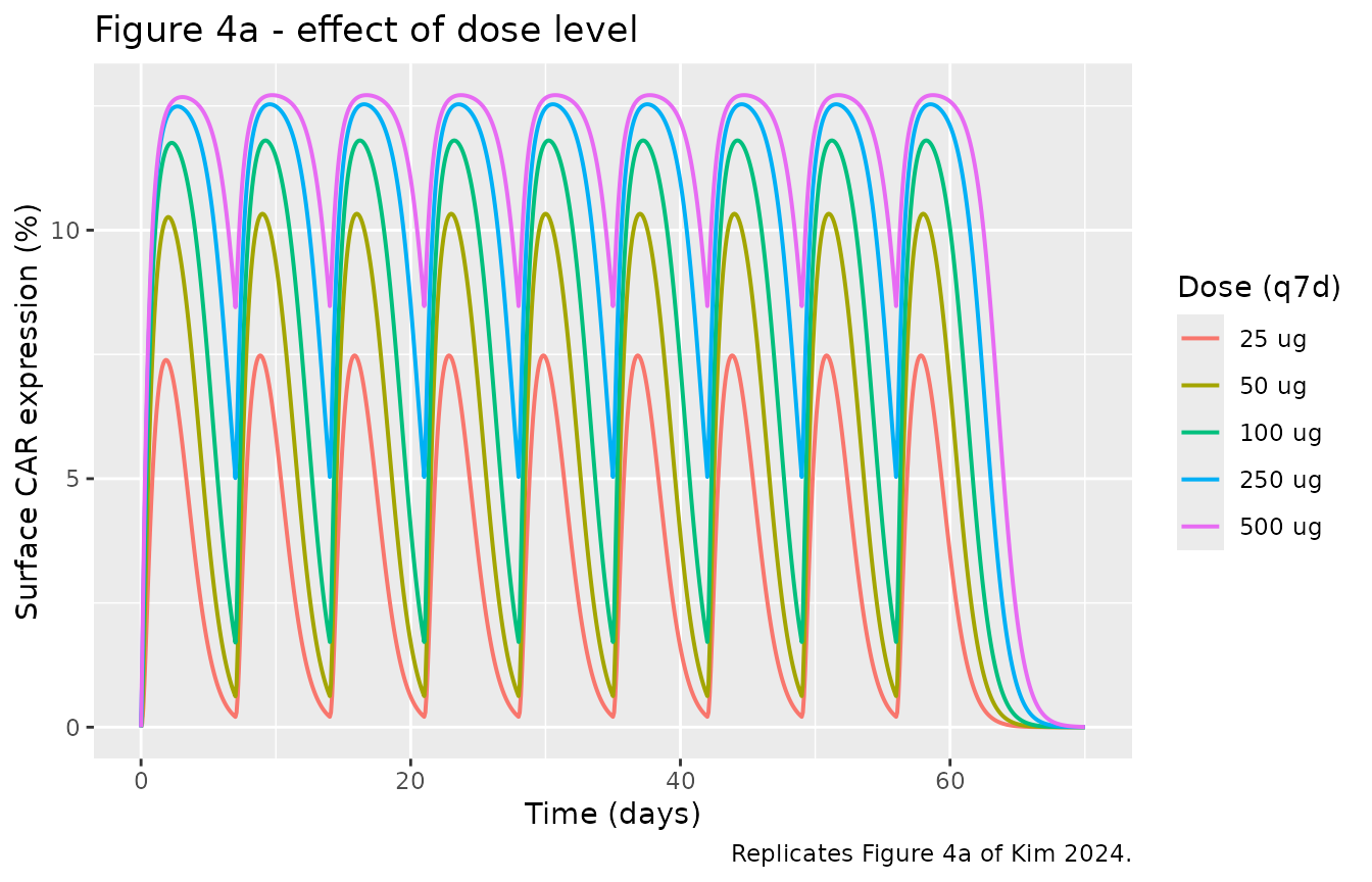
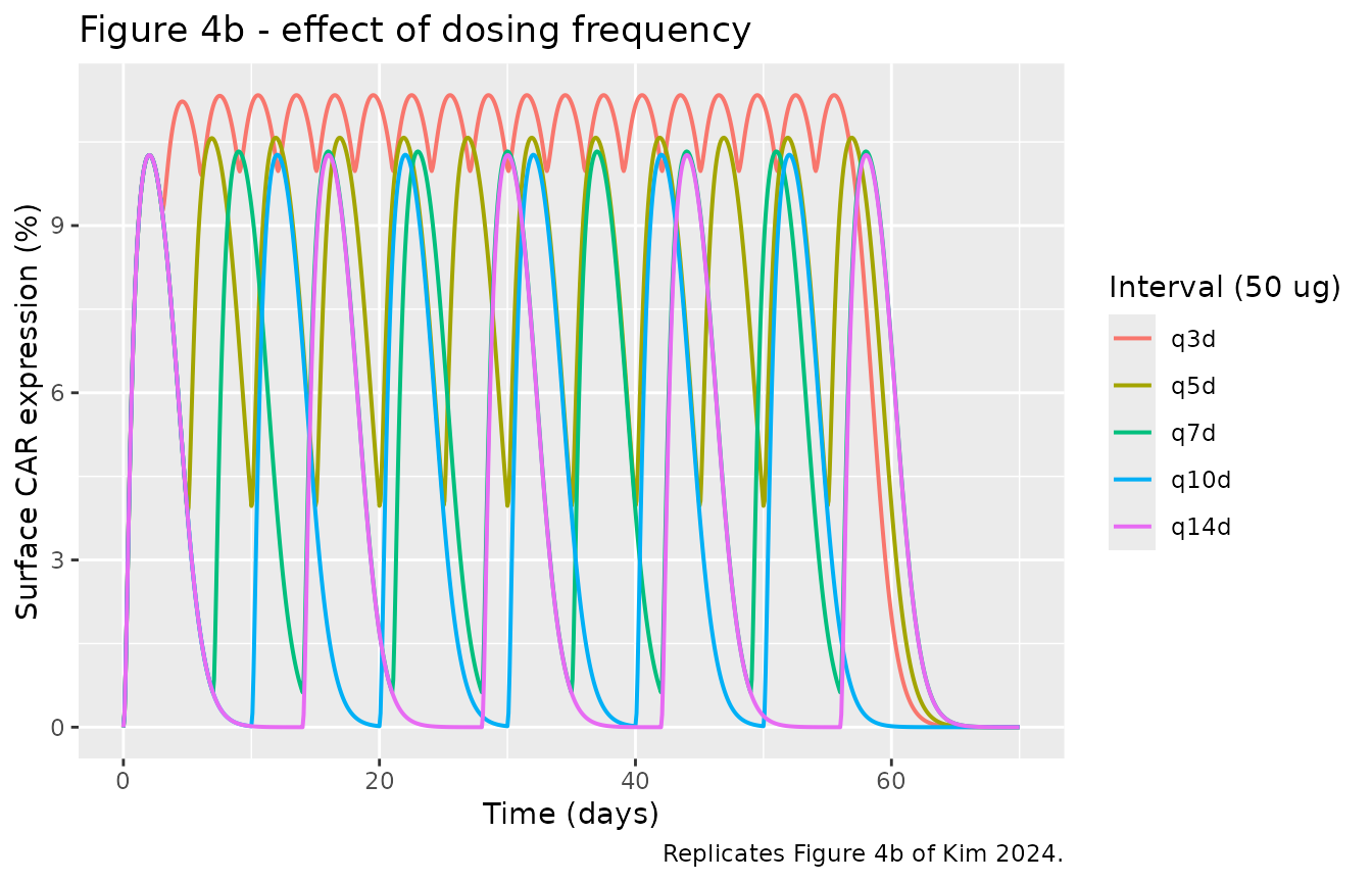
Impact of dose and dosing frequency (replicates Figure 4)
The model supports the paper’s dose-optimisation simulations. Each
arm is a typical-value profile. To compare arms fairly, every arm is
dosed across the same fixed active window (dosing_days) and
then followed into washout, rather than for a fixed number of doses: a
fixed dose count would let the shorter interval finish dosing - and
begin washing out - while a longer interval is still being dosed, making
any steady-state comparison meaningless. The steady-state metrics below
are taken from a window (days 28-49) that falls inside the active-dosing
phase of every arm.
sim_regimen <- function(dose_ug, interval_days, dosing_days = 56, horizon_days = 70) {
  amt <- (dose_ug * 1e-6 / mw) / (V1_mL * 1e-3) * 1e12
  interval_h <- interval_days * 24
  dose_times <- seq(0, dosing_days * 24, by = interval_h)
  ev <- et(amt = amt, cmt = "mrna_central", time = dose_times) |>
    et(seq(0, horizon_days * 24, by = 2))
  s <- rxSolve(m_mo, ev, returnType = "data.frame")
  s$dose_ug <- dose_ug
  s$interval_days <- interval_days
  s
}

# Steady-state window inside the active-dosing phase of every arm (q3d-q14d).
ss_window <- function(df) df[df$time >= 28 * 24 & df$time <= 49 * 24, ]
# 4a: vary dose level (0.5x to 10x of 50 ug), fixed weekly interval.
doses <- c(0.5, 1, 2, 5, 10) * 50
f4a <- bind_rows(lapply(doses, sim_regimen, interval_days = 7))
#> ℹ omega/sigma items treated as zero: 'etalec50', 'etalhill', 'etalkdeg'
#> ℹ omega/sigma items treated as zero: 'etalec50', 'etalhill', 'etalkdeg'
#> ℹ omega/sigma items treated as zero: 'etalec50', 'etalhill', 'etalkdeg'
#> ℹ omega/sigma items treated as zero: 'etalec50', 'etalhill', 'etalkdeg'
#> ℹ omega/sigma items treated as zero: 'etalec50', 'etalhill', 'etalkdeg'
f4a$arm <- factor(paste0(f4a$dose_ug, " ug"), levels = paste0(doses, " ug"))

ggplot(f4a, aes(time / 24, carexpr, colour = arm)) +
  geom_line(linewidth = 0.7) +
  labs(
    x = "Time (days)", y = "Surface CAR expression (%)",
    colour = "Dose (q7d)", title = "Figure 4a - effect of dose level",
    caption = "Replicates Figure 4a of Kim 2024."
  )
# 4b: vary dosing interval (q3d to q14d), fixed 50 ug dose.
intervals <- c(3, 5, 7, 10, 14)
f4b <- bind_rows(lapply(intervals, function(iv) sim_regimen(50, iv)))
#> ℹ omega/sigma items treated as zero: 'etalec50', 'etalhill', 'etalkdeg'
#> ℹ omega/sigma items treated as zero: 'etalec50', 'etalhill', 'etalkdeg'
#> ℹ omega/sigma items treated as zero: 'etalec50', 'etalhill', 'etalkdeg'
#> ℹ omega/sigma items treated as zero: 'etalec50', 'etalhill', 'etalkdeg'
#> ℹ omega/sigma items treated as zero: 'etalec50', 'etalhill', 'etalkdeg'
f4b$arm <- factor(paste0("q", f4b$interval_days, "d"), levels = paste0("q", intervals, "d"))

ggplot(f4b, aes(time / 24, carexpr, colour = arm)) +
  geom_line(linewidth = 0.7) +
  labs(
    x = "Time (days)", y = "Surface CAR expression (%)",
    colour = "Interval (50 ug)", title = "Figure 4b - effect of dosing frequency",
    caption = "Replicates Figure 4b of Kim 2024."
  )
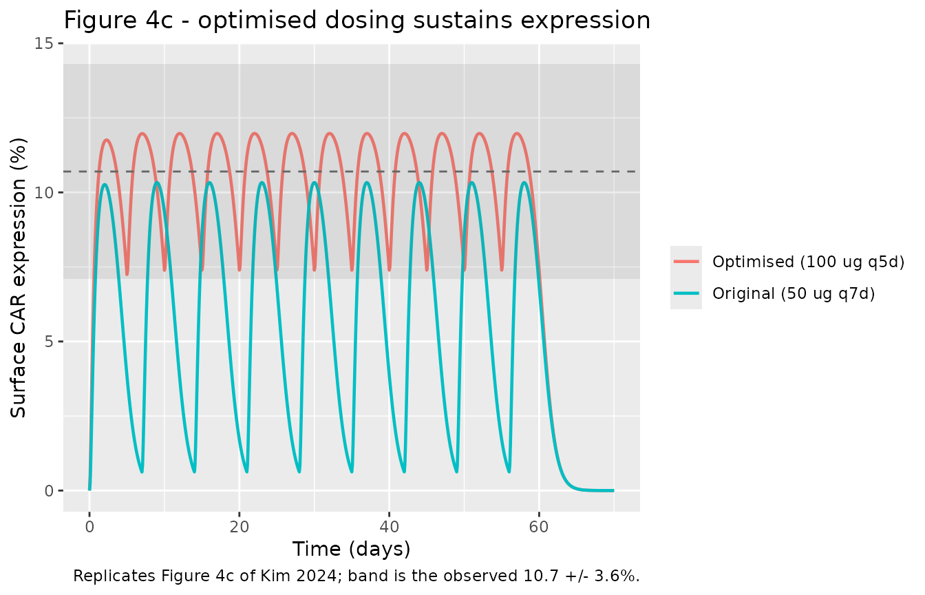
# 4c: proposed optimised regimen (2x dose = 100 ug, q5d) vs the original.
f4c <- bind_rows(
  sim_regimen(50, 7) |> mutate(arm = "Original (50 ug q7d)"),
  sim_regimen(100, 5) |> mutate(arm = "Optimised (100 ug q5d)")
)
#> ℹ omega/sigma items treated as zero: 'etalec50', 'etalhill', 'etalkdeg'
#> ℹ omega/sigma items treated as zero: 'etalec50', 'etalhill', 'etalkdeg'

ggplot(f4c, aes(time / 24, carexpr, colour = arm)) +
  geom_line(linewidth = 0.8) +
  geom_hline(yintercept = 10.7, linetype = "dashed", colour = "grey40") +
  annotate("rect",
    xmin = -Inf, xmax = Inf, ymin = 10.7 - 3.6, ymax = 10.7 + 3.6,
    alpha = 0.12, fill = "grey40"
  ) +
  labs(
    x = "Time (days)", y = "Surface CAR expression (%)",
    colour = NULL, title = "Figure 4c - optimised dosing sustains expression",
    caption = "Replicates Figure 4c of Kim 2024; band is the observed 10.7 +/- 3.6%."
  )
# All metrics are taken from the steady-state window (days 28-49), which is
# inside the active-dosing phase of every arm.

# Figure 4a: higher dose raises the steady-state peak (monotone).
peak_by_dose <- sapply(doses, function(d) max(ss_window(f4a[f4a$dose_ug == d, ])$carexpr))
stopifnot(all(diff(peak_by_dose) > 0))

# Figure 4b: a shorter interval shrinks the peak-trough swing and raises the
# trough (sustained expression), exactly the paper's qualitative finding.
swing_by_interval <- sapply(intervals, function(iv) {
  w <- ss_window(f4b[f4b$interval_days == iv, ])$carexpr
  max(w) - min(w)
})
trough_by_interval <- sapply(intervals, function(iv) min(ss_window(f4b[f4b$interval_days == iv, ])$carexpr))
stopifnot(
  all(diff(swing_by_interval) > 0), # swing grows as the interval lengthens
  all(diff(trough_by_interval) < 0) # trough falls as the interval lengthens
)

# Figure 4c: the optimised arm (2x dose, q5d) holds its steady-state trough well
# above the original arm's trough.
opt_ss <- ss_window(f4c[f4c$arm == "Optimised (100 ug q5d)", ])
orig_ss <- ss_window(f4c[f4c$arm == "Original (50 ug q7d)", ])
stopifnot(min(opt_ss$carexpr) > min(orig_ss$carexpr))
c(
  opt_trough = round(min(opt_ss$carexpr), 2),
  orig_trough = round(min(orig_ss$carexpr), 2)
)
#>  opt_trough orig_trough
#>        7.39        0.63
Mass-balance and steady-state sanity
With no dose, every state holds at zero (the biological baseline before transfection): there is no endogenous production term.
s0 <- rxSolve(m_mo, et(seq(0, 30 * 24, by = 24)), returnType = "data.frame")
#> ℹ omega/sigma items treated as zero: 'etalec50', 'etalhill', 'etalkdeg'
stopifnot(all(abs(s0$carexpr) < 1e-8), all(abs(s0$mrna_free) < 1e-8))
The NP-receptor complex and free intracellular mRNA are strictly non-negative and the binding reaction conserves mRNA between the media/central pool and the complex (no mRNA is created by binding):
Assumptions and deviations
-
carexpris a paper-mechanistic PD output. The surface-CAR-expression readout is a percent, not a drug concentration, so it is declared as a paper-specific compartment and observed directly.checkModelConventions()flags a single non-canonical observation variable; the maintainers kept the descriptive name rather than minting a new canonical PD-output state for a single paper, and note it here. A future CAR-mRNA model reusing this endpoint would be a reason to canonicalise it. -
Free receptor held constant. Following the paper’s
parsimonious model, the free CD8 receptor concentration
rtotis a fixed constant (2483 pM, Table 2) rather than a depleting state. Appendix S1 Eq. 1 works a related figure of 497 pM for 1e9 cells/L; the tabulated 2483 pM used in both the fits and the Appendix S2 simulation code corresponds to a roughly 5-fold higher effective receptor density, so the Table 2 value is carried here. -
States are concentrations; the dose is given in pM.
The paper’s ODEs are dimensionally consistent only with concentration
states, so
V1enters only through the dose-mass-to-concentration conversion (shown above) and thertotderivation, not as an ODE term. -
Final estimates from Table 2. Where the Appendix S2
simulation code and Table 2 differ slightly, the published Table 2
estimates are used:
knp(0.086 in Table 2 vs 0.091 in the code) andec50in vivo (124 vs 124.17). The difference does not change the reproduced 10.7% result materially. -
In vitro IIV on
kdeg_trans. The 30% IIV listed forkdeg_transin the in vitro column was estimated in the separate one-compartment relative-mRNA submodel (Appendix S1 Eq. 6) and then fixed; it is not carried into the surface-CAR model, wherekdeg_transis a fixed constant. - Typical-value simulations. The figures use random-effects-zeroed (typical-value) profiles, matching the fitted-profile figures of the paper; the estimated IIV terms are small (CV < 13% on the in vivo parameters) and do not drive the reported mean.
- No correction notice for this article was found as of 2026-11-01. ```