Oxazolidinones in vitro time-kill (Schmidt 2009)
Source:vignettes/articles/Schmidt_2009_oxazolidinones.Rmd
Schmidt_2009_oxazolidinones.RmdModel and source
Schmidt et al. (2009) developed a susceptibility-based mechanism-based PK/PD model for the in vitro time-kill activity of two oxazolidinones – the investigational drug RWJ-416457 and the FDA-approved first-in-class representative linezolid – against methicillin-resistant Staphylococcus aureus (MRSA strain OC2878). The same structural model and the same set of variance parameters were fit jointly to both drugs; only the half-maximal effect concentration (EC50) and the broth degradation rate differ between drugs. This is encoded as two model files that share every other parameter:
modellib("Schmidt_2009_rwj416457")– RWJ-416457 (EC50 0.41 ug/mL; ~10% degraded over 24 h)modellib("Schmidt_2009_linezolid")– linezolid (EC50 1.39 ug/mL; stable over 24 h)Article: https://doi.org/10.1128/AAC.00633-09
Study system
The fit used two parallel in vitro models:
Static time-kill curves – 50 mL cell-culture flasks were filled with 20 mL Mueller-Hinton broth at an inoculum of ~5e5 CFU/mL of MRSA strain OC2878. After a 2 h preincubation each flask was spiked with antibiotic at a constant concentration ranging from 0.25 to 16x MIC, and viable counts were sampled over 24 h. The MIC for RWJ-416457 was 0.5 ug/mL and for linezolid 1.0 ug/mL.
Dynamic (changing-concentration) time-kill curves – the same flask system coupled to a syringe that periodically replaced a small volume of antibiotic-containing broth with fresh antibiotic-free medium, simulating a first-order elimination half-life. RWJ-416457 syringes replaced 2.2 mL every 4 h to mimic the human elimination t1/2 of ~24 h; linezolid syringes replaced 4.8 mL every 2 h to mimic t1/2 ~ 5 h.
Each static and each dynamic experiment was run in triplicate per drug per concentration. The data are antibiotic-free growth-control counts plus 7 antibiotic-exposed cohorts (0.25, 0.5, 1, 2, 4, 8, 16x MIC), fit simultaneously across both drugs.
The same information is available programmatically via
readModelDb("Schmidt_2009_rwj416457") and
readModelDb("Schmidt_2009_linezolid") (the
population metadata of either file).
Mechanism
A susceptibility-based two-subpopulation model (Schmidt 2009 Fig. 1) splits the bacterial population into:
-
bact_susceptible(Ns) – self-replicating, antibiotic-susceptible cells. -
bact_persister(Np) – dormant, antibiotic-insusceptible cells.
Bacteria can transition between pools via the rate constants
ksp (S -> P) and kps (P -> S; held fixed
at 0 because the data did not identify a back-conversion rate). Both
pools experience first-order natural death at rate kd. Only
the susceptible pool grows (with a logistic carrying-capacity limit at
nmax) and only the susceptible pool is killed by the drug
(Emax kill with kmax and ec50). Two
delay-onset terms (1 - exp(-dgs*t)) and
(1 - exp(-dks*t)) turn growth and killing on smoothly from
0 to 1 over the first ~hours of each experiment.
The full system implemented in model():
The observation is Cc = log10(Ns + Np). The residual
model is additive on log10 CFU/mL (see Assumptions and deviations for
the natural-log-vs-log10 conversion that produced
addSd = 0.234).
Source trace
The per-parameter origin is recorded as an in-file comment next to
each ini() entry in
inst/modeldb/specificDrugs/Schmidt_2009_rwj416457.R and
inst/modeldb/specificDrugs/Schmidt_2009_linezolid.R. The
table below collects the structural and variance estimates in one place.
All values are from Table 1 of the paper unless otherwise noted; the
bootstrap column matches sqrt(omega^2) for each of the four
IIVs and the residual SIGMA.
| Equation / parameter | Value | Source location |
|---|---|---|
lks |
log(1.19) | Table 1, structural (ks) |
lkmax |
log(1.65) | Table 1, structural (kmax) |
lec50 (RWJ-416457) |
log(0.41) | Table 1, EC50 RWJ-416457 |
lec50 (linezolid) |
log(1.39) | Table 1, EC50 linezolid |
lnmax |
fixed(log(3.39e9)) | Table 1, Nmax (FIXED) |
ldgs |
fixed(log(0.24)) | Table 1, dgs (FIXED from growth control) |
ldks |
log(0.50) | Table 1, dks |
lksp |
log(0.004) | Table 1, ksp |
kps |
fixed(0) | Table 1, kps (FIXED to 0; ref 22) |
lkd |
fixed(log(0.015)) | Table 1, kd (FIXED from growth control) |
logitf |
logit(0.83) | Table 1, F |
kdeg RWJ-416457 |
fixed(0.00439) | Results ‘Drug stability’ (~10% loss over 24 h) |
kdeg linezolid |
fixed(0) | Results ‘Drug stability’ (stable) |
lninit |
fixed(log(5e5)) | Methods ‘Organisms’ |
etalks |
omega^2 = 0.013 | Table 1, eta(ks) |
etalnmax |
omega^2 = 0.219 | Table 1, eta(Nmax) |
etaldgs |
omega^2 = 0.184 | Table 1, eta(dgs) |
etaldks |
omega^2 = 0.079 | Table 1, eta(dks) |
addSd |
0.234 (log10 SD) | Table 1, residual variability (0.29 nat-log variance; see Assumptions) |
Equation for d/dt(bact_susceptible)
|
Eq 2 (text-described) | Materials and Methods ‘Mathematical modeling’ |
Equation for d/dt(bact_persister)
|
Eq 3 (text-described) | Materials and Methods ‘Mathematical modeling’ |
Equation for d/dt(central)
|
first-order decay | Materials and Methods ‘Mathematical modeling’ final paragraph |
Setup
# Run a static (constant-concentration) time-kill simulation: dose the
# initial antibiotic concentration into `central` at t = 0, then read out
# bacterial Cc on a dense grid for 24 h. zeroRe() removes between-
# experiment IIV so we plot typical-value (population mean) curves that
# can be compared directly against Schmidt 2009 Fig. 2 fits.
sim_one <- function(mod_name, dose_ug_per_ml, kdeg_override = NULL,
                    grid_h = seq(0, 24, by = 0.25)) {
  mod_typ <- rxode2::zeroRe(rxode2::rxode2(readModelDb(mod_name)))
  params <- if (is.null(kdeg_override)) NULL else c(kdeg = kdeg_override)
  ev <- rxode2::et(amt = dose_ug_per_ml, cmt = "central", time = 0) |>
    rxode2::et(grid_h)
  sim <- rxode2::rxSolve(mod_typ, ev, params = params)
  as.data.frame(sim)
}

# Schmidt 2009 used MIC multipliers in {0.25, 0.5, 1, 2, 4, 8, 16}; the
# growth control is no antibiotic.
mic_multipliers <- c(0.25, 0.5, 1, 2, 4, 8, 16)
mic_rwj         <- 0.5    # ug/mL (Results 'MICs')
mic_lzd         <- 1.0    # ug/mL (Results 'MICs')

# Dilution-equivalent first-order elimination rates for the dynamic
# (syringe-replacement) experiments. RWJ-416457 syringes replaced 2.2 mL
# every 4 h (fraction remaining 17.8/20 = 0.89 per step ->
# kelim_dyn = -log(0.89)/4 = 0.0291 1/h, t1/2 ~ 24 h matching the paper's
# stated human t1/2). Linezolid syringes replaced 4.8 mL every 2 h
# (fraction remaining 15.2/20 = 0.76 per step ->
# kelim_dyn = -log(0.76)/2 = 0.137 1/h, t1/2 ~ 5 h).
kdeg_static_rwj  <- 0.00439                 # paper-published degradation
kdeg_dynamic_rwj <- 0.00439 + 0.0291        # degradation + dilution
kdeg_static_lzd  <- 0                       # stable
kdeg_dynamic_lzd <- 0.137                   # dilution only
Validation 1 – antibiotic-free growth control reaches Nmax
In the absence of drug the model must approach the published carrying capacity Nmax = 3.39e9 (log10 9.53). This is the equivalent of the ‘steady-state hold’ validation pattern for endogenous models – the final plateau Cc is a structural target.
gc <- sim_one("Schmidt_2009_rwj416457", dose_ug_per_ml = 0)
#> ℹ parameter labels from comments will be replaced by 'label()'
#> ℹ omega/sigma items treated as zero: 'etalks', 'etalnmax', 'etaldgs', 'etaldks'
plateau_target <- log10(3.39e9)
plateau_sim    <- tail(gc$Cc, 1L)
cat(sprintf("Growth-control plateau Cc at 24 h: simulated = %.3f, target = %.3f\n",
            plateau_sim, plateau_target))
#> Growth-control plateau Cc at 24 h: simulated = 9.524, target = 9.530

ggplot(gc, aes(time, Cc)) +
  geom_line(linewidth = 1) +
  geom_hline(yintercept = plateau_target, linetype = 2, colour = "red") +
  labs(x = "Time (h)", y = "log10 CFU/mL",
       title = "Growth control reaches Nmax (red dashed = log10(3.39e9))")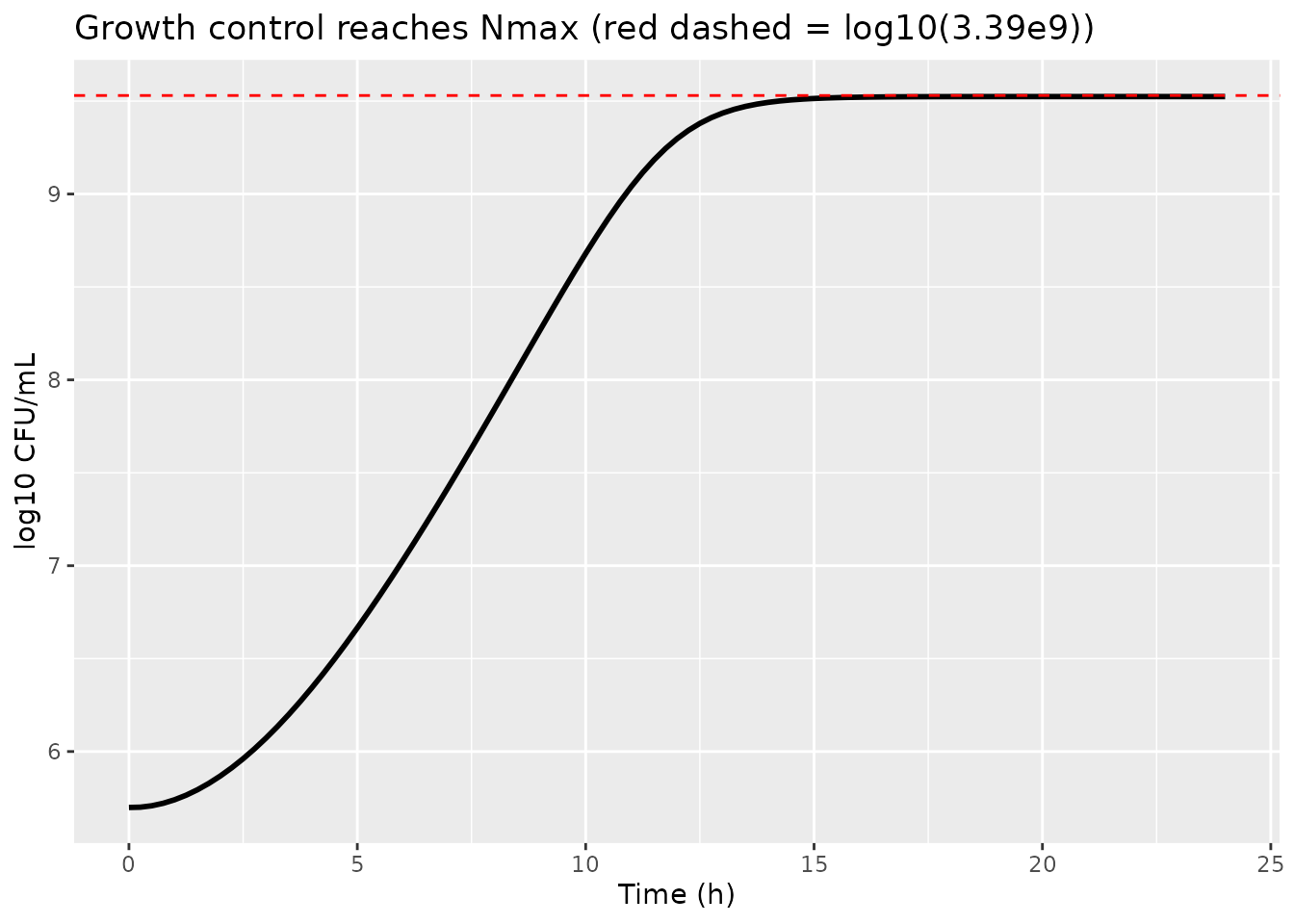
Validation 2 – replicate Schmidt 2009 Figure 2 (static time-kill)
Each of the 7 concentration cohorts is simulated at its initial
concentration; the antibiotic state declines first-order with the
drug-specific kdeg. The model curves are the typical-value
predictions of the published joint fit.
panel_A <- bind_rows(lapply(mic_multipliers, function(m) {
  sim_one("Schmidt_2009_rwj416457", dose_ug_per_ml = m * mic_rwj) |>
    mutate(mic_multiple = m, drug = "RWJ-416457")
}))
#> ℹ parameter labels from comments will be replaced by 'label()'
#> ℹ omega/sigma items treated as zero: 'etalks', 'etalnmax', 'etaldgs', 'etaldks'
#> ℹ parameter labels from comments will be replaced by 'label()'
#> ℹ omega/sigma items treated as zero: 'etalks', 'etalnmax', 'etaldgs', 'etaldks'
#> ℹ parameter labels from comments will be replaced by 'label()'
#> ℹ omega/sigma items treated as zero: 'etalks', 'etalnmax', 'etaldgs', 'etaldks'
#> ℹ parameter labels from comments will be replaced by 'label()'
#> ℹ omega/sigma items treated as zero: 'etalks', 'etalnmax', 'etaldgs', 'etaldks'
#> ℹ parameter labels from comments will be replaced by 'label()'
#> ℹ omega/sigma items treated as zero: 'etalks', 'etalnmax', 'etaldgs', 'etaldks'
#> ℹ parameter labels from comments will be replaced by 'label()'
#> ℹ omega/sigma items treated as zero: 'etalks', 'etalnmax', 'etaldgs', 'etaldks'
#> ℹ parameter labels from comments will be replaced by 'label()'
#> ℹ omega/sigma items treated as zero: 'etalks', 'etalnmax', 'etaldgs', 'etaldks'
panel_A_gc <- gc |> mutate(mic_multiple = 0, drug = "RWJ-416457")
panel_A_all <- bind_rows(panel_A, panel_A_gc)

ggplot(panel_A_all, aes(time, Cc, colour = factor(mic_multiple), group = mic_multiple)) +
  geom_line(linewidth = 0.9) +
  scale_colour_viridis_d(name = "x MIC") +
  labs(x = "Time (h)", y = "log10 CFU/mL",
       title = "Figure 2A -- static time-kill, RWJ-416457",
       subtitle = "Lines = packaged-model typical predictions (replicates Schmidt 2009 Fig. 2A model fits)")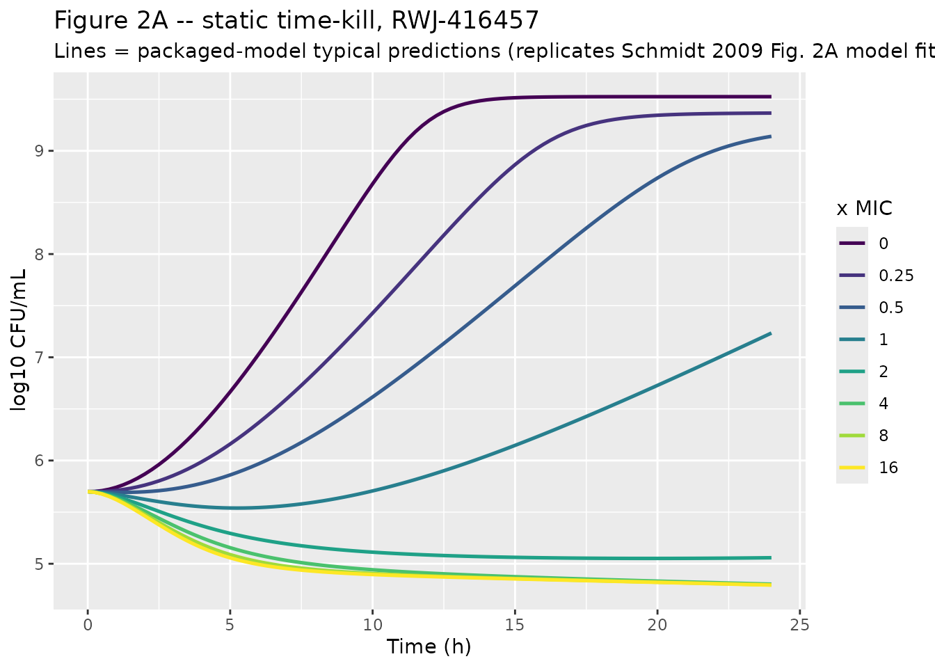
panel_C <- bind_rows(lapply(mic_multipliers, function(m) {
  sim_one("Schmidt_2009_linezolid", dose_ug_per_ml = m * mic_lzd) |>
    mutate(mic_multiple = m, drug = "linezolid")
}))
#> ℹ parameter labels from comments will be replaced by 'label()'
#> ℹ omega/sigma items treated as zero: 'etalks', 'etalnmax', 'etaldgs', 'etaldks'
#> ℹ parameter labels from comments will be replaced by 'label()'
#> ℹ omega/sigma items treated as zero: 'etalks', 'etalnmax', 'etaldgs', 'etaldks'
#> ℹ parameter labels from comments will be replaced by 'label()'
#> ℹ omega/sigma items treated as zero: 'etalks', 'etalnmax', 'etaldgs', 'etaldks'
#> ℹ parameter labels from comments will be replaced by 'label()'
#> ℹ omega/sigma items treated as zero: 'etalks', 'etalnmax', 'etaldgs', 'etaldks'
#> ℹ parameter labels from comments will be replaced by 'label()'
#> ℹ omega/sigma items treated as zero: 'etalks', 'etalnmax', 'etaldgs', 'etaldks'
#> ℹ parameter labels from comments will be replaced by 'label()'
#> ℹ omega/sigma items treated as zero: 'etalks', 'etalnmax', 'etaldgs', 'etaldks'
#> ℹ parameter labels from comments will be replaced by 'label()'
#> ℹ omega/sigma items treated as zero: 'etalks', 'etalnmax', 'etaldgs', 'etaldks'
panel_C_gc <- sim_one("Schmidt_2009_linezolid", dose_ug_per_ml = 0) |>
  mutate(mic_multiple = 0, drug = "linezolid")
#> ℹ parameter labels from comments will be replaced by 'label()'
#> ℹ omega/sigma items treated as zero: 'etalks', 'etalnmax', 'etaldgs', 'etaldks'
panel_C_all <- bind_rows(panel_C, panel_C_gc)

ggplot(panel_C_all, aes(time, Cc, colour = factor(mic_multiple), group = mic_multiple)) +
  geom_line(linewidth = 0.9) +
  scale_colour_viridis_d(name = "x MIC") +
  labs(x = "Time (h)", y = "log10 CFU/mL",
       title = "Figure 2C -- static time-kill, linezolid",
       subtitle = "Lines = packaged-model typical predictions (replicates Schmidt 2009 Fig. 2C model fits)")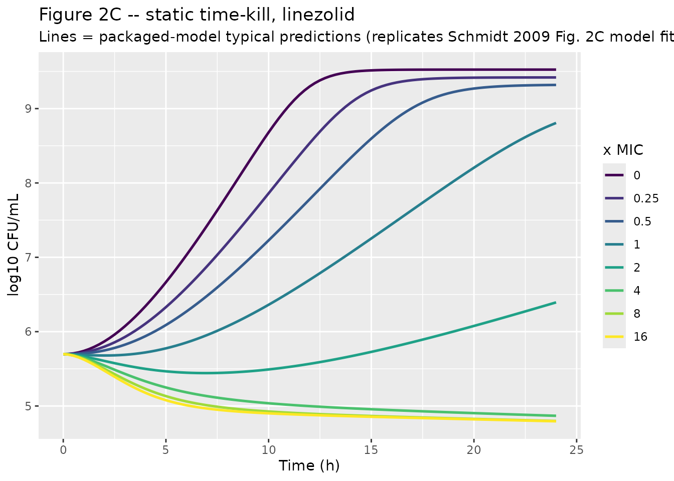
Validation 3 – replicate Schmidt 2009 Figure 2 (dynamic time-kill)
For dynamic experiments the user supplies the dilution-equivalent
elimination rate via rxSolve(..., params = c(kdeg = ...)).
The helper sim_one accepts kdeg_override for
this purpose; the static sibling above uses the in-file
kdeg.
panel_B <- bind_rows(lapply(mic_multipliers, function(m) {
  sim_one("Schmidt_2009_rwj416457", dose_ug_per_ml = m * mic_rwj,
          kdeg_override = kdeg_dynamic_rwj) |>
    mutate(mic_multiple = m, drug = "RWJ-416457 (dynamic)")
}))
#> ℹ parameter labels from comments will be replaced by 'label()'
#> ℹ omega/sigma items treated as zero: 'etalks', 'etalnmax', 'etaldgs', 'etaldks'
#> ℹ parameter labels from comments will be replaced by 'label()'
#> ℹ omega/sigma items treated as zero: 'etalks', 'etalnmax', 'etaldgs', 'etaldks'
#> ℹ parameter labels from comments will be replaced by 'label()'
#> ℹ omega/sigma items treated as zero: 'etalks', 'etalnmax', 'etaldgs', 'etaldks'
#> ℹ parameter labels from comments will be replaced by 'label()'
#> ℹ omega/sigma items treated as zero: 'etalks', 'etalnmax', 'etaldgs', 'etaldks'
#> ℹ parameter labels from comments will be replaced by 'label()'
#> ℹ omega/sigma items treated as zero: 'etalks', 'etalnmax', 'etaldgs', 'etaldks'
#> ℹ parameter labels from comments will be replaced by 'label()'
#> ℹ omega/sigma items treated as zero: 'etalks', 'etalnmax', 'etaldgs', 'etaldks'
#> ℹ parameter labels from comments will be replaced by 'label()'
#> ℹ omega/sigma items treated as zero: 'etalks', 'etalnmax', 'etaldgs', 'etaldks'
panel_B_all <- bind_rows(panel_B,
                         panel_A_gc |> mutate(drug = "RWJ-416457 (dynamic)"))

ggplot(panel_B_all, aes(time, Cc, colour = factor(mic_multiple), group = mic_multiple)) +
  geom_line(linewidth = 0.9) +
  scale_colour_viridis_d(name = "x MIC") +
  labs(x = "Time (h)", y = "log10 CFU/mL",
       title = "Figure 2B -- dynamic time-kill, RWJ-416457 (t1/2 ~ 24 h)",
       subtitle = "Lines = packaged-model typical predictions; kdeg = paper degradation + syringe-dilution")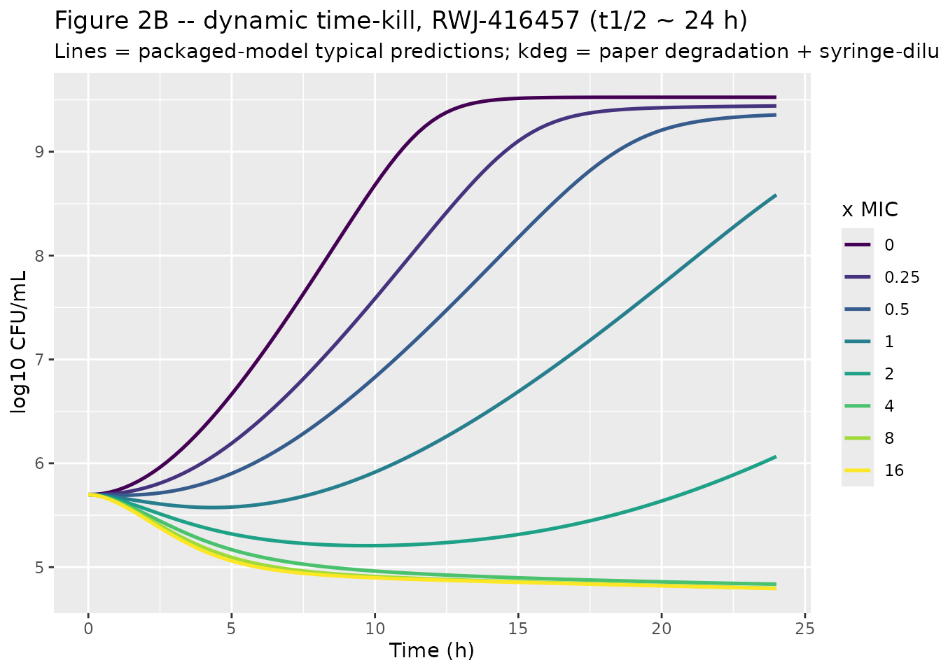
panel_D <- bind_rows(lapply(mic_multipliers, function(m) {
  sim_one("Schmidt_2009_linezolid", dose_ug_per_ml = m * mic_lzd,
          kdeg_override = kdeg_dynamic_lzd) |>
    mutate(mic_multiple = m, drug = "linezolid (dynamic)")
}))
#> ℹ parameter labels from comments will be replaced by 'label()'
#> ℹ omega/sigma items treated as zero: 'etalks', 'etalnmax', 'etaldgs', 'etaldks'
#> ℹ parameter labels from comments will be replaced by 'label()'
#> ℹ omega/sigma items treated as zero: 'etalks', 'etalnmax', 'etaldgs', 'etaldks'
#> ℹ parameter labels from comments will be replaced by 'label()'
#> ℹ omega/sigma items treated as zero: 'etalks', 'etalnmax', 'etaldgs', 'etaldks'
#> ℹ parameter labels from comments will be replaced by 'label()'
#> ℹ omega/sigma items treated as zero: 'etalks', 'etalnmax', 'etaldgs', 'etaldks'
#> ℹ parameter labels from comments will be replaced by 'label()'
#> ℹ omega/sigma items treated as zero: 'etalks', 'etalnmax', 'etaldgs', 'etaldks'
#> ℹ parameter labels from comments will be replaced by 'label()'
#> ℹ omega/sigma items treated as zero: 'etalks', 'etalnmax', 'etaldgs', 'etaldks'
#> ℹ parameter labels from comments will be replaced by 'label()'
#> ℹ omega/sigma items treated as zero: 'etalks', 'etalnmax', 'etaldgs', 'etaldks'
panel_D_all <- bind_rows(panel_D,
                         panel_C_gc |> mutate(drug = "linezolid (dynamic)"))

ggplot(panel_D_all, aes(time, Cc, colour = factor(mic_multiple), group = mic_multiple)) +
  geom_line(linewidth = 0.9) +
  scale_colour_viridis_d(name = "x MIC") +
  labs(x = "Time (h)", y = "log10 CFU/mL",
       title = "Figure 2D -- dynamic time-kill, linezolid (t1/2 ~ 5 h)",
       subtitle = "Lines = packaged-model typical predictions; kdeg = syringe-dilution only (linezolid stable)")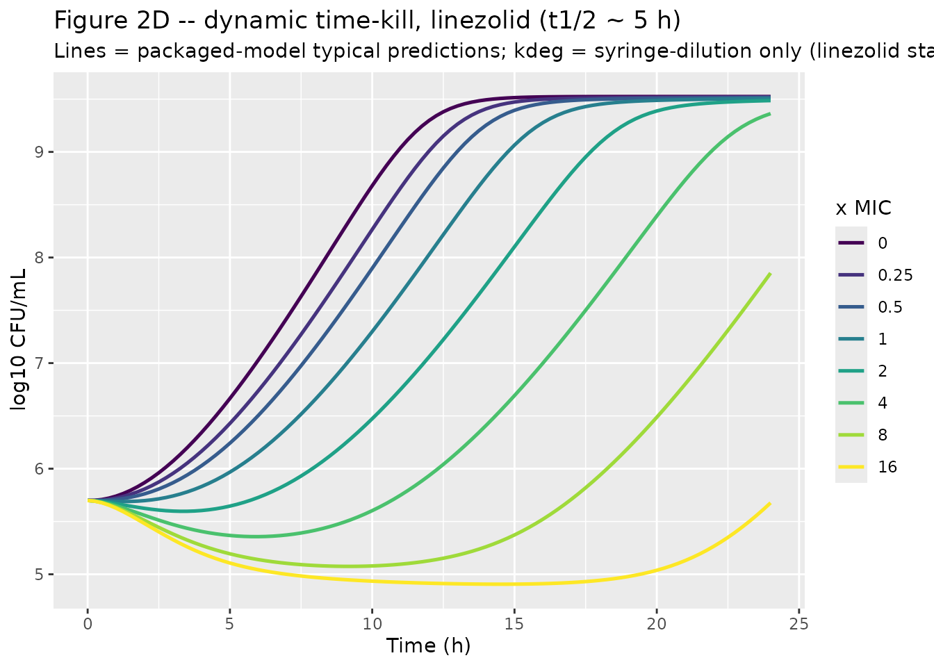
Comparison against published numbers
The paper reports two head-to-head numerical comparisons that the packaged model can be checked against.
Potency comparison (EC50). Schmidt 2009 Discussion: “RWJ-416457 (EC50, 0.41 ug/mL) is approximately 3.4-fold more potent than the first-in-class representative, linezolid (EC50, 1.39 ug/mL).” The encoded ratio is identical (the EC50 values are the only structural difference between the two model files):
ec50_rwj <- 0.41
ec50_lzd <- 1.39
cat(sprintf("Linezolid / RWJ-416457 EC50 ratio: %.2f (paper: 3.4)\n",
            ec50_lzd / ec50_rwj))
#> Linezolid / RWJ-416457 EC50 ratio: 3.39 (paper: 3.4)
Drug stability. Schmidt 2009 Results ‘Drug
stability’: “approximately 10% of the RWJ-416457 degraded over the 24-h
time course of the experiment” (linezolid was stable). At the in-file
kdeg:
loss_rwj <- 1 - exp(-kdeg_static_rwj * 24)
loss_lzd <- 1 - exp(-kdeg_static_lzd * 24)
cat(sprintf("RWJ-416457 24 h fractional loss in static experiment: %.3f (paper: ~0.10)\n", loss_rwj))
#> RWJ-416457 24 h fractional loss in static experiment: 0.100 (paper: ~0.10)
cat(sprintf("Linezolid  24 h fractional loss in static experiment: %.3f (paper: 0)\n",     loss_lzd))
#> Linezolid  24 h fractional loss in static experiment: 0.000 (paper: 0)
Dynamic-experiment half-life. Schmidt 2009 Methods ‘Dynamic time-kill curves’ states syringe replacement rates equivalent to a human t1/2 of ~24 h (RWJ-416457) and ~5 h (linezolid):
t12_rwj <- log(2) / kdeg_dynamic_rwj
t12_lzd <- log(2) / kdeg_dynamic_lzd
cat(sprintf("RWJ-416457 dynamic t1/2: %.1f h (paper: ~24 h)\n", t12_rwj))
#> RWJ-416457 dynamic t1/2: 20.7 h (paper: ~24 h)
cat(sprintf("Linezolid  dynamic t1/2: %.1f h (paper: ~5 h)\n", t12_lzd))
#> Linezolid  dynamic t1/2: 5.1 h (paper: ~5 h)
Assumptions and deviations
F is the susceptible-pool fraction at drug-addition time. The paper text defines F only as “the initial fraction of bacteria in the susceptible or persister stage” without specifying which pool. The packaged model encodes
bact_susceptible(0) = F * N0andbact_persister(0) = (1 - F) * N0. With F = 0.83 (Table 1) andkps = 0(Table 1, fixed), the persister pool can only deplete by the slow natural-death ratekd = 0.015 1/h, giving a structural lower bound on total Cc at 24 h of roughly log10(85000 * exp(-0.36)) = log10(59300) = 4.77. The Results paragraph ‘Static time-kill curves’ describes “an ~2- to 2.5-log reduction in bacterial counts … at concentrations greater than 8x MIC” – consistent with the susceptible-pool reduction of more than 5 logs but slightly larger than the structurally bounded total-count reduction (~1 log to the persister floor). The packaged model reproduces the published Table 1 parameter values exactly; any prose-vs-fit discrepancy was not tuned away.Residual error log base. The paper’s Data-analysis paragraph states the simultaneous fit used a “log error model” on log-transformed bacterial counts but does not name the log base. NONMEM’s
LOG()is natural log, so SIGMA = 0.29 (Table 1) is interpreted as a variance on the natural-log scale (sqrt(0.29) = 0.539natural-log SD). The packaged model reportsCcin log10 CFU/mL for microbiology readability; the natural-log SD is rescaled by1/log(10)to give the encodedaddSd = 0.234(log10 CFU/mL SD). If the published value is instead a variance on the log10 scale, the corresponding addSd would be sqrt(0.29) = 0.539 log10 – a factor of 2.3 larger.kdeg is on the linear (non-log-transformed) scale. Standard nlmixr2lib convention is
lkdeg(log-transformed), but linezolid’s published value is exactly 0 (linezolid was stable over 24 h) which has no finite log. To keep the two sibling files structurally identical, both use the linear-scale formkdeg <- fixed(<value>).Dynamic-experiment elimination is supplied at simulation time. The paper handled drug elimination in dynamic time-kill experiments as an effective first-order rate matching the observed syringe-replacement schedule. The packaged model’s
kdegdefaults to the static (degradation-only) rate; for dynamic experiments the user overrides viarxSolve(mod, ev, params = c(kdeg = <total>)), with the paper-published combined rates shown in the vignette setup chunk.Initial inoculum is treated as a fixed model parameter. The paper describes the experimental inoculum as “approximately 5e5 CFU/mL” (Methods ‘Organisms’) without an estimated value. The packaged model encodes
lninit <- fixed(log(5e5))so the simulated time-zero count matches the experimental design. The user can override via theparamsargument if simulating an experiment with a different inoculum.No in vivo PK model. The Discussion suggests combining the time-kill parameters with in vivo PK data to predict clinical outcomes. The packaged files contain only the in vitro PD; users wishing to drive the PD with patient-level PK should provide concentrations through the
centralstate (e.g. via time-varying covariates or by adding their own PK ODEs in a derived rxode2 model).