Siponimod (Huth 2019) • nlmixr2lib

Model and source

Citation: Huth F, Gardin A, Umehara K, He H. (2019). Prediction of the Impact of Cytochrome P450 2C9 Genotypes on the Drug-Drug Interaction Potential of Siponimod With Physiologically-Based Pharmacokinetic Modeling: A Comprehensive Approach for Drug Label Recommendations. Clin Pharmacol Ther 106(5):1113-1124. doi:10.1002/cpt.1547.
Article: https://doi.org/10.1002/cpt.1547 (PMC6851657, open access)

Siponimod is an oral, selective sphingosine-1-phosphate receptor 1 and 5 modulator approved for relapsing forms of multiple sclerosis. It is cleared almost entirely by hepatic oxidative metabolism, and CYP2C9 carries about 80% of that clearance, so the CYP2C9 diplotype moves siponimod exposure roughly fivefold. Huth 2019 built a full-PBPK model in the Simcyp Population-based Simulator (V16) to predict how seven CYP3A4 and CYP2C9 perpetrators interact with siponimod in each of the six clinically relevant CYP2C9 diplotypes. Those predictions are the basis of the approved label’s drug-interaction and genotype-specific dosing language.

What this model file is, and what it is not

This is a compartmental reduction of the published Simcyp model, not a port of it. The Simcyp full-PBPK distribution model resolves every organ separately, and its per-organ partition coefficients, volumes and blood flows are platform database outputs that appear in no publication. What made the reduction possible is that Huth 2019 is unusually explicit about where its two load-bearing disposition inputs came from, and neither is a platform prediction:

Table 5 footnote f: the Vss of 1.45 L/kg is the observed mean Vss from the intravenous arm, converted on the 80.08 kg mean body weight of the study subjects. The Kp scalar of 0.574 is described as “optimized”, i.e. the platform’s predicted partition coefficients were rescaled to this observed volume.
Table 5 footnote g: the retrograde clearance calculation was driven by the observed geometric mean CL of 3.12 L/h.

So the aggregate volume and the clearance are clinical measurements, and the enzyme split, absorption and first-pass terms are all printed. Only two numbers are missing, and both are aggregates that no whole-body model publishes: a central volume and a distribution clearance.

What is encoded here:

two-compartment oral disposition with first-order absorption and a lag;
clearance split into a CYP2C9 arm, a CYP3A4 arm and a residual arm, from the fractions metabolised in Table 5 section 4;
the six CYP2C9 diplotypes, as a relative activity on the CYP2C9 arm;
all seven perpetrators, each as relative CYP3A4 and CYP2C9 activities that scale the matching clearance arm together with gut-wall and hepatic first-pass extraction.

What is not encoded:

the Simcyp whole-body mass-balance equations and the per-organ physiology;
the perpetrators’ own mechanistic parameters. Every perpetrator except fluconazole is a Simcyp V16 compound-file entry with nothing printed, and even fluconazole’s entry is a platform file with one revised Ki. This model therefore encodes each perpetrator’s published exposure ratio, not the platform’s inhibition or induction mechanism, so it cannot extrapolate to a dose or regimen the paper did not simulate;
the Simcyp virtual-population variability (about 48% CV on AUC and 20% on Cmax in Table 1), which is driven by unpublished demographic and enzyme-abundance distributions. This is a typical-value model with no etas and no residual error.

How the two missing numbers were obtained

The central volume vc and the intercompartmental clearance q were solved so that the reduction reproduces exactly two statistics from Huth 2019 Table 1: the predicted single-oral-dose Tmax of 3.45 h and the predicted Cmax of 7.76 ng/mL per mg. The peripheral volume is then not free at all – it is the printed Vss minus vc.

A one-compartment reduction was tried first and rejected: with V = Vss it over-predicts the printed Tmax by 86% (6.41 h against 3.45 h), because siponimod has a real distribution phase that a single compartment cannot express. The printed Vss, clearance and terminal half-life cannot by themselves supply a second compartment, because log(2) * Vss / CL is 25.8 h against a printed terminal half-life of 25.5 h – the three numbers sit at the one-compartment limit and leave no information about how the volume is partitioned.

Everything downstream of those two numbers is a gate, not a fit. The strongest is the intravenous arm of Table 1, which was held out entirely.

Population

Every simulation in Huth 2019 used the Simcyp healthy-volunteer population, justified in the Methods by a population-PK finding of no clinically relevant PK difference between healthy volunteers and patients with multiple sclerosis. The clinical data behind the model come from five studies: a single-ascending-dose study (0.1 to 75 mg, n = 6 to 8 per dose), a multiple-ascending-dose study (0.3 to 20 mg once daily for 28 days, n = 6 to 9 per dose), an absolute-bioavailability study (n = 15) that supplied the paired 0.25 mg intravenous and oral arms and hence both disposition anchors, a CYP2C9 pharmacogenetic study that supplied the genotype PK of Table 2 and the fluconazole interaction, and a dedicated rifampin interaction study.

The mean body weight of the study subjects was 80.08 kg (Table 5 footnote f). In the white population the six diplotypes occur at roughly 62-65% (*1/*1), 20-24% (*1/*2), 9-12% (*1/*3), 1-2% (*2/*2), 1.4-1.7% (*2/*3) and 0.3-0.4% (*3/*3) (Introduction). Observed genotype PK was available only for *1/*1 (n = 12), *2/*3 (n = 6) and *3/*3 (n = 6).

Source trace

Provenance of every model quantity.
Quantity	Value	Source location
ka	0.687 1/h	Table 5, ‘Absorption rate constant’, fn d (popPK)
Lag time	1.5 h	Table 5, ‘Lag time (h)’, optimized
f_a (dosage-form availability)	0.91	Table 5, ‘Fraction available from dosage form’, fn c
Vss	1.45 L/kg	Table 5, fn f: observed mean Vss on 80.08 kg
Body weight	80.08 kg	Table 5 fn f
CL (CYP2C91/1)	3.12 L/h	Table 5 fn g; = 0.25 mg / 80.1 ng*h/mL, Table 1 i.v. observed
Renal CL / biliary CL	0 / 0	Table 5 section 5, fn i (mass-balance study)
fm CYP2C9 / CYP3A4 by genotype	6 pairs	Table 5 section 4, ‘CL int (allelic CYP2C9x/y)’ rows
Absolute bioavailability	0.849	Table 1: predicted oral AUCinf 69.7 / i.v. AUCinf 82.1
Hepatic blood flow QH	90 L/h	NOT printed; standard value, see Assumptions
vc, q	43.72 L, 30.02 L/h	BACK-SOLVED from Table 1 oral Tmax 3.45 h and Cmax 7.76 ng/mL/mg
vp	72.39 L	Vss - vc; not free
Perpetrator relative activities	10 values	BACK-SOLVED from the 42 AUC ratios of Table 3

Single-dose verification against Table 1

mod <- readModelDb("Huth_2019_siponimod")

conmed_cols <- c("CONMED_ITRACONAZOLE", "CONMED_KETOCONAZOLE", "CONMED_ERYTHROMYCIN",
                 "CONMED_FLUCONAZOLE", "CONMED_FLUVOXAMINE", "CONMED_RIFAMPICIN",
                 "CONMED_EFV")

# Covariate block for one arm: diplotype allele counts plus the seven
# perpetrator flags (all zero = siponimod alone).
cov_block <- function(d, s1, s2, s3, modulator = NA_character_) {
  d$CYP2C9_S1_COUNT <- s1
  d$CYP2C9_S2_COUNT <- s2
  d$CYP2C9_S3_COUNT <- s3
  for (nm in conmed_cols) {
    d[[nm]] <- if (!is.na(modulator) && nm == modulator) 1 else 0
  }
  d
}

sd_arms <- tibble::tribble(
  ~arm,            ~dose, ~iv,
  "0.1 mg p.o.",     0.1, FALSE,
  "0.3 mg p.o.",     0.3, FALSE,
  "1 mg p.o.",       1.0, FALSE,
  "2.5 mg p.o.",     2.5, FALSE,
  "5 mg p.o.",       5.0, FALSE,
  "10 mg p.o.",     10.0, FALSE,
  "17.5 mg p.o.",   17.5, FALSE,
  "25 mg p.o.",     25.0, FALSE,
  "75 mg p.o.",     75.0, FALSE,
  "0.25 mg p.o.",    0.25, FALSE,
  "0.25 mg i.v.",    0.25, TRUE
)

# Observations sit on the `central` ODE state; rxode2 returns the algebraic
# observable Cc as a column at those rows.
make_sd_arm <- function(i) {
  a <- sd_arms[i, ]
  tgrid <- sort(unique(c(seq(0, 24, by = 0.05), seq(24, 600, by = 1))))
  ev <- if (a$iv) {
    rxode2::et(amt = a$dose, dur = 2.92, cmt = "central")
  } else {
    rxode2::et(amt = a$dose, cmt = "depot")
  }
  ev <- rxode2::et(ev, tgrid, cmt = "central")
  d <- as.data.frame(ev)
  d$id <- i
  d$arm <- a$arm
  d$dose <- a$dose
  cov_block(d, 2, 0, 0)
}

sd_events <- dplyr::bind_rows(lapply(seq_len(nrow(sd_arms)), make_sd_arm))

sd_sim <- rxode2::rxSolve(mod, sd_events, keep = c("arm", "dose")) |>
  as.data.frame()
#> Warning: multi-subject simulation without without 'omega'
stopifnot(nrow(sd_sim) > 0, !all(is.na(sd_sim$Cc)), all(sd_sim$Cc >= 0, na.rm = TRUE))

The intravenous arm is the important one. Huth 2019 reports an observed Tmax of 2.92 h with a zero-width range for the 0.25 mg intravenous dose, which identifies it as a 2.92 h infusion; that arm was not used to obtain vc or q.

sd_nca_in <- sd_sim |>
  dplyr::filter(!is.na(Cc)) |>
  dplyr::select(id, time, Cc, arm, dose)

sd_nca_in <- dplyr::bind_rows(
  sd_nca_in,
  sd_nca_in |> dplyr::distinct(id, arm, dose) |> dplyr::mutate(time = 0, Cc = 0)
) |>
  dplyr::distinct(id, arm, time, .keep_all = TRUE) |>
  dplyr::arrange(id, time)

sd_conc <- PKNCA::PKNCAconc(sd_nca_in, Cc ~ time | arm + id)
sd_dose <- PKNCA::PKNCAdose(
  sd_events |> dplyr::filter(evid %in% c(1, 101)) |>
    dplyr::select(id, time, amt, arm, dose) |>
    dplyr::distinct(id, arm, .keep_all = TRUE),
  amt ~ time | arm + id
)
sd_intervals <- data.frame(
  start = 0, end = Inf,
  cmax = TRUE, tmax = TRUE, aucinf.obs = TRUE, half.life = TRUE, aucpext.obs = TRUE
)
sd_res <- PKNCA::pk.nca(PKNCA::PKNCAdata(sd_conc, sd_dose, intervals = sd_intervals))

sd_wide <- as.data.frame(sd_res) |>
  dplyr::select(arm, PPTESTCD, PPORRES) |>
  tidyr::pivot_wider(names_from = PPTESTCD, values_from = PPORRES)
# The observation window must be long enough that extrapolation is negligible,
# otherwise the AUC comparison measures the window rather than the model.
stopifnot(max(sd_wide$aucpext.obs, na.rm = TRUE) < 2)

# Huth 2019 Table 1, "Predicted" columns.
published_sd <- tibble::tribble(
  ~arm,            ~cmax, ~tmax, ~aucinf.obs, ~half.life,
  "0.1 mg p.o.",    0.78,  3.45,      29.1,      25.6,
  "0.3 mg p.o.",    2.33,  3.45,      87.2,      25.6,
  "1 mg p.o.",      7.76,  3.45,     291,        25.6,
  "2.5 mg p.o.",   19.4,   3.45,     727,        25.6,
  "5 mg p.o.",     38.8,   3.45,    1454,        25.6,
  "10 mg p.o.",    77.7,   3.45,    2908,        25.6,
  "17.5 mg p.o.", 136,     3.45,    5088,        25.6,
  "25 mg p.o.",   194,     3.45,    7269,        25.6,
  "75 mg p.o.",   582,     3.45,   21807,        25.6,
  "0.25 mg p.o.",   1.88,  3.25,      69.7,      25.5,
  "0.25 mg i.v.",   3.02,  3.00,      82.1,      25.5
)

sd_cmp <- nlmixr2lib::ncaComparisonTable(
  simulated     = sd_res,
  reference     = published_sd,
  by            = "arm",
  params        = c("cmax", "tmax", "aucinf.obs", "half.life"),
  units         = c(cmax = "ng/mL", tmax = "h", aucinf.obs = "ng*h/mL", half.life = "h"),
  tolerance_pct = 20
)

kbl(
  sd_cmp,
  caption = paste("Reduction vs the Simcyp model's own predicted values",
                  "(Huth 2019 Table 1). * marks a difference over 20%.")
)

Reduction vs the Simcyp model’s own predicted values (Huth 2019 Table 1). * marks a difference over 20%.
NCA parameter	arm	Reference	Simulated	% diff
Cmax (ng/mL)	0.1 mg p.o.	0.78	0.776	-0.5%
Cmax (ng/mL)	0.3 mg p.o.	2.33	2.33	-0.1%
Cmax (ng/mL)	1 mg p.o.	7.76	7.76	+0.0%
Cmax (ng/mL)	2.5 mg p.o.	19.4	19.4	+0.0%
Cmax (ng/mL)	5 mg p.o.	38.8	38.8	+0.0%
Cmax (ng/mL)	10 mg p.o.	77.7	77.6	-0.1%
Cmax (ng/mL)	17.5 mg p.o.	136	136	-0.1%
Cmax (ng/mL)	25 mg p.o.	194	194	+0.0%
Cmax (ng/mL)	75 mg p.o.	582	582	+0.0%
Cmax (ng/mL)	0.25 mg p.o.	1.88	1.94	+3.2%
Cmax (ng/mL)	0.25 mg i.v.	3.02	2.97	-1.6%
Tmax (h)	0.1 mg p.o.	3.45	3.45	+0.0%
Tmax (h)	0.3 mg p.o.	3.45	3.45	+0.0%
Tmax (h)	1 mg p.o.	3.45	3.45	+0.0%
Tmax (h)	2.5 mg p.o.	3.45	3.45	+0.0%
Tmax (h)	5 mg p.o.	3.45	3.45	+0.0%
Tmax (h)	10 mg p.o.	3.45	3.45	+0.0%
Tmax (h)	17.5 mg p.o.	3.45	3.45	+0.0%
Tmax (h)	25 mg p.o.	3.45	3.45	+0.0%
Tmax (h)	75 mg p.o.	3.45	3.45	+0.0%
Tmax (h)	0.25 mg p.o.	3.25	3.45	+6.2%
Tmax (h)	0.25 mg i.v.	3	2.9	-3.3%
AUC0-∞ (obs) (ng*h/mL)	0.1 mg p.o.	29.1	27.2	-6.5%
AUC0-∞ (obs) (ng*h/mL)	0.3 mg p.o.	87.2	81.6	-6.4%
AUC0-∞ (obs) (ng*h/mL)	1 mg p.o.	291	272	-6.5%
AUC0-∞ (obs) (ng*h/mL)	2.5 mg p.o.	727	680	-6.4%
AUC0-∞ (obs) (ng*h/mL)	5 mg p.o.	1450	1360	-6.4%
AUC0-∞ (obs) (ng*h/mL)	10 mg p.o.	2910	2720	-6.4%
AUC0-∞ (obs) (ng*h/mL)	17.5 mg p.o.	5090	4760	-6.4%
AUC0-∞ (obs) (ng*h/mL)	25 mg p.o.	7270	6800	-6.4%
AUC0-∞ (obs) (ng*h/mL)	75 mg p.o.	21800	20400	-6.4%
AUC0-∞ (obs) (ng*h/mL)	0.25 mg p.o.	69.7	68	-2.4%
AUC0-∞ (obs) (ng*h/mL)	0.25 mg i.v.	82.1	80.1	-2.4%
t½ (h)	0.1 mg p.o.	25.6	26.8	+4.8%
t½ (h)	0.3 mg p.o.	25.6	26.8	+4.8%
t½ (h)	1 mg p.o.	25.6	26.8	+4.8%
t½ (h)	2.5 mg p.o.	25.6	26.8	+4.8%
t½ (h)	5 mg p.o.	25.6	26.8	+4.8%
t½ (h)	10 mg p.o.	25.6	26.8	+4.8%
t½ (h)	17.5 mg p.o.	25.6	26.8	+4.8%
t½ (h)	25 mg p.o.	25.6	26.8	+4.8%
t½ (h)	75 mg p.o.	25.6	26.8	+4.8%
t½ (h)	0.25 mg p.o.	25.5	26.8	+5.2%
t½ (h)	0.25 mg i.v.	25.5	26.8	+5.2%

The worst deviation across all 44 cells is 6.5%. Two systematic offsets are worth naming rather than tuning away:

AUC on the 0.1-75 mg ladder is about 6.5% low. That ladder’s own predicted AUC implies a CL/F of 3.44 L/h, whereas this model uses the CL of 3.12 L/h that Table 5 footnote g names as the model input, with the bioavailability of 0.849 that Table 1 predicts, giving CL/F = 3.67. The discrepancy is between two different Simcyp virtual populations in the same table (n = 340 for the ladder, n = 100 for the 0.25 mg arms), not between the reduction and the model. Against the 0.25 mg arms, which use the same population as the inputs, the AUC agreement is within 2.5%.
Intravenous Cmax lands at 2.99 ng/mL against 3.02 predicted (-1.1%). This is the out-of-sample corroboration of vc and q: a two-compartment model fitted only to an oral peak time and height has no obligation to reproduce the height of an intravenous infusion peak, and it does.

# Replicates Figure 2a of Huth 2019: simulated mean siponimod concentration vs
# time after a single 0.1 mg oral dose in the CYP2C9*1/*1 genotype.
sd_sim |>
  dplyr::filter(arm %in% c("0.1 mg p.o.", "1 mg p.o.", "75 mg p.o."), time > 0, time <= 400) |>
  dplyr::mutate(arm = factor(arm, levels = c("0.1 mg p.o.", "1 mg p.o.", "75 mg p.o."))) |>
  ggplot(aes(time, Cc, colour = arm)) +
  geom_line(linewidth = 0.8) +
  scale_y_log10() +
  scale_colour_manual(values = c("#2E7D32", "#EF6C00", "#6A1B9A")) +
  labs(x = "Time (h)", y = "Siponimod plasma concentration (ng/mL)", colour = NULL,
       title = "Single oral doses, CYP2C9*1/*1",
       caption = "Replicates Figure 2a and 2b of Huth 2019 (typical-value profiles).") +
  theme_bw() +
  theme(legend.position = "top")
#> Warning in scale_y_log10(): log-10 transformation introduced infinite values.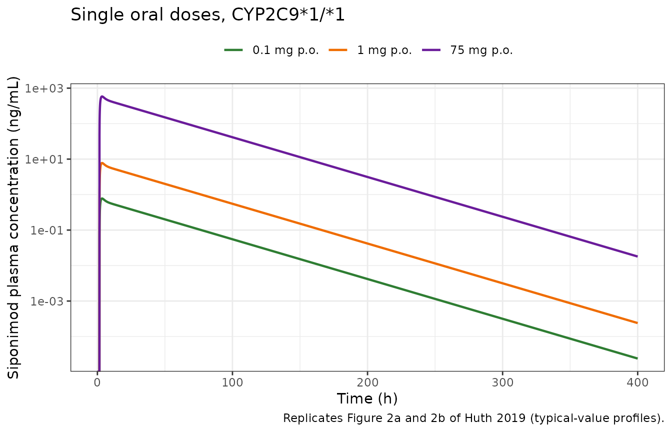

Genotype verification against Table 2

Table 2 is a genuine out-of-sample gate. Nothing in it was used to build the model: the genotype clearances come from the fraction-metabolised pairs in Table 5, and vc / q come from the *1/*1 dose ladder in Table 1.

genos <- tibble::tribble(
  ~arm,      ~s1, ~s2, ~s3,
  "*1/*1",    2,   0,   0,
  "*1/*2",    1,   1,   0,
  "*1/*3",    1,   0,   1,
  "*2/*2",    0,   2,   0,
  "*2/*3",    0,   1,   1,
  "*3/*3",    0,   0,   2
)

make_geno_arm <- function(i) {
  g <- genos[i, ]
  tgrid <- sort(unique(c(seq(0, 24, by = 0.05), seq(24, 1500, by = 2))))
  ev <- rxode2::et(amt = 0.25, cmt = "depot") |>
    rxode2::et(tgrid, cmt = "central")
  d <- as.data.frame(ev)
  d$id <- i
  d$arm <- g$arm
  cov_block(d, g$s1, g$s2, g$s3)
}
geno_events <- dplyr::bind_rows(lapply(seq_len(nrow(genos)), make_geno_arm))
geno_sim <- rxode2::rxSolve(mod, geno_events, keep = "arm") |> as.data.frame()
#> Warning: multi-subject simulation without without 'omega'
stopifnot(nrow(geno_sim) > 0, all(geno_sim$Cc >= 0, na.rm = TRUE))

geno_nca_in <- geno_sim |>
  dplyr::filter(!is.na(Cc)) |>
  dplyr::select(id, time, Cc, arm)
geno_nca_in <- dplyr::bind_rows(
  geno_nca_in,
  geno_nca_in |> dplyr::distinct(id, arm) |> dplyr::mutate(time = 0, Cc = 0)
) |>
  dplyr::distinct(id, arm, time, .keep_all = TRUE) |>
  dplyr::arrange(id, time)

geno_res <- PKNCA::pk.nca(PKNCA::PKNCAdata(
  PKNCA::PKNCAconc(geno_nca_in, Cc ~ time | arm + id),
  PKNCA::PKNCAdose(
    geno_events |> dplyr::filter(evid %in% c(1, 101)) |>
      dplyr::select(id, time, amt, arm) |> dplyr::distinct(id, arm, .keep_all = TRUE),
    amt ~ time | arm + id
  ),
  intervals = data.frame(start = 0, end = Inf, cmax = TRUE, aucinf.obs = TRUE,
                         half.life = TRUE, aucpext.obs = TRUE)
))
#> Warning: aucpext is typically only calculated when aucinf is greater than
#> auclast.

published_geno <- tibble::tribble(
  ~arm,     ~cmax, ~aucinf.obs, ~half.life,
  "*1/*1",   1.90,     70.6,      25.5,
  "*1/*2",   1.92,     76.2,      27.4,
  "*1/*3",   1.99,    117,        41.1,
  "*2/*2",   1.97,     98.7,      34.9,
  "*2/*3",   2.02,    142,        49.2,
  "*3/*3",   2.10,    348,       118
)

geno_cmp <- nlmixr2lib::ncaComparisonTable(
  simulated     = geno_res,
  reference     = published_geno,
  by            = "arm",
  params        = c("cmax", "aucinf.obs", "half.life"),
  units         = c(cmax = "ng/mL", aucinf.obs = "ng*h/mL", half.life = "h"),
  tolerance_pct = 20
)
kbl(
  geno_cmp,
  caption = paste("CYP2C9 diplotype gate: reduction vs Huth 2019 Table 2",
                  "predicted values, single 0.25 mg oral dose.",
                  "Nothing in this table was used to build the model.")
)

CYP2C9 diplotype gate: reduction vs Huth 2019 Table 2 predicted values, single 0.25 mg oral dose. Nothing in this table was used to build the model.
NCA parameter	arm	Reference	Simulated	% diff
Cmax (ng/mL)	1/1	1.9	1.94	+2.1%
Cmax (ng/mL)	1/2	1.92	1.95	+1.8%
Cmax (ng/mL)	1/3	1.99	2.02	+1.6%
Cmax (ng/mL)	2/2	1.97	2	+1.4%
Cmax (ng/mL)	2/3	2.02	2.04	+1.1%
Cmax (ng/mL)	3/3	2.1	2.11	+0.5%
AUC0-∞ (obs) (ng*h/mL)	1/1	70.6	68	-3.6%
AUC0-∞ (obs) (ng*h/mL)	1/2	76.2	73.7	-3.3%
AUC0-∞ (obs) (ng*h/mL)	1/3	117	113	-3.3%
AUC0-∞ (obs) (ng*h/mL)	2/2	98.7	95.8	-2.9%
AUC0-∞ (obs) (ng*h/mL)	2/3	142	136	-4.5%
AUC0-∞ (obs) (ng*h/mL)	3/3	348	329	-5.6%
t½ (h)	1/1	25.5	27	+5.9%
t½ (h)	1/2	27.4	29	+6.0%
t½ (h)	1/3	41.1	43.4	+5.5%
t½ (h)	2/2	34.9	37.1	+6.2%
t½ (h)	2/3	49.2	51.6	+4.8%
t½ (h)	3/3	118	122	+3.4%

Worst deviation 6.2% across an exposure range that spans a factor of five and a half-life range that spans a factor of four and a half. That the *3/*3 half-life of 118 h falls out of the printed Vss and the printed fraction-metabolised pair, with no adjustment, is the single strongest evidence that the fm-based genotype derivation is what the authors actually did.

There is one internal check worth stating explicitly, because it is free and it validates the derivation before any simulation happens. Huth 2019 Table 5 prints only fm CYP2C9 and fm CYP3A4 for each genotype, and those two do not sum to 1. Fixing the CYP3A4 clearance arm at its genotype-invariant value of 0.546 L/h implies a residual fraction for every genotype; adding it back closes each row:

Each genotype row of Table 5 closes to 1.000.
Genotype	fm CYP2C9	fm CYP3A4	CL (L/h)	fm other (implied)	Sum
1/1	0.804	0.175	3.120	0.021	1.000
1/2	0.788	0.189	2.889	0.023	1.000
1/3	0.678	0.287	1.902	0.034	0.999
2/2	0.727	0.244	2.238	0.029	1.000
2/3	0.616	0.343	1.592	0.041	1.000
3/3	0.074	0.822	0.664	0.099	0.995

Drug-interaction verification against Table 3

Table 3 gives, for every combination of seven perpetrators and six diplotypes, a steady-state AUC ratio and a Cmax ratio: 84 numbers. Each perpetrator’s relative enzyme activities were back-solved from that perpetrator’s six AUC ratios only – one free number for the four perpetrators the paper classifies as CYP3A4-selective, two for the three it classifies as dual. All 42 Cmax ratios were held out.

perps <- tibble::tribble(
  ~label,          ~col,                   ~class,
  "Itraconazole",  "CONMED_ITRACONAZOLE",  "Strong CYP3A4 inhibitor",
  "Ketoconazole",  "CONMED_KETOCONAZOLE",  "Strong CYP3A4 inhibitor",
  "Erythromycin",  "CONMED_ERYTHROMYCIN",  "Moderate CYP3A4 inhibitor",
  "Fluconazole",   "CONMED_FLUCONAZOLE",   "Moderate CYP3A4/2C9 inhibitor",
  "Fluvoxamine",   "CONMED_FLUVOXAMINE",   "Weak CYP3A4/2C9 inhibitor",
  "Rifampicin",    "CONMED_RIFAMPICIN",    "Strong CYP3A4/moderate 2C9 inducer",
  "Efavirenz",     "CONMED_EFV",           "Moderate CYP3A4 inducer"
)

# Huth 2019 dosed to steady state over 90 days for the inhibitors. The dose
# cancels out of a ratio in a linear model; 2 mg once daily is the approved
# maintenance dose.
NDOSE <- 90L
tau <- 24
ddi_grid <- tidyr::expand_grid(
  gi = seq_len(nrow(genos)),
  pi = c(0L, seq_len(nrow(perps)))
)

make_ddi_arm <- function(k) {
  gi <- ddi_grid$gi[k]
  pi <- ddi_grid$pi[k]
  g <- genos[gi, ]
  modulator <- if (pi == 0L) NA_character_ else perps$col[pi]
  # Observe only the final dosing interval; everything before it is burn-in.
  tgrid <- seq((NDOSE - 1) * tau, NDOSE * tau, by = 0.1)
  ev <- rxode2::et(amt = 2, cmt = "depot", ii = tau, addl = NDOSE - 1L) |>
    rxode2::et(tgrid, cmt = "central")
  d <- as.data.frame(ev)
  d$id <- k
  d$geno <- g$arm
  d$perp <- if (pi == 0L) "None" else perps$label[pi]
  cov_block(d, g$s1, g$s2, g$s3, modulator)
}
ddi_events <- dplyr::bind_rows(lapply(seq_len(nrow(ddi_grid)), make_ddi_arm))

ddi_sim <- rxode2::rxSolve(mod, ddi_events, keep = c("geno", "perp")) |>
  as.data.frame()
#> Warning: multi-subject simulation without without 'omega'
stopifnot(nrow(ddi_sim) > 0, all(ddi_sim$Cc >= 0, na.rm = TRUE))

ddi_nca_in <- ddi_sim |>
  dplyr::filter(!is.na(Cc)) |>
  dplyr::select(id, time, Cc, geno, perp) |>
  dplyr::arrange(id, time)

ddi_res <- PKNCA::pk.nca(PKNCA::PKNCAdata(
  PKNCA::PKNCAconc(ddi_nca_in, Cc ~ time | geno + perp + id),
  PKNCA::PKNCAdose(
    ddi_events |> dplyr::filter(evid %in% c(1, 101)) |>
      dplyr::mutate(time = (NDOSE - 1) * tau) |>
      dplyr::select(id, time, amt, geno, perp) |>
      dplyr::distinct(id, .keep_all = TRUE),
    amt ~ time | geno + perp + id
  ),
  intervals = data.frame(
    start = (NDOSE - 1) * tau, end = NDOSE * tau, cmax = TRUE, auclast = TRUE
  )
))

ddi_wide <- as.data.frame(ddi_res) |>
  dplyr::select(geno, perp, PPTESTCD, PPORRES) |>
  tidyr::pivot_wider(names_from = PPTESTCD, values_from = PPORRES)

ddi_ratio <- ddi_wide |>
  dplyr::filter(perp != "None") |>
  dplyr::left_join(
    ddi_wide |> dplyr::filter(perp == "None") |>
      dplyr::select(geno, cmax0 = cmax, auc0 = auclast),
    by = "geno"
  ) |>
  dplyr::mutate(aucr = auclast / auc0, cmaxr = cmax / cmax0)

ddi_cmp <- ddi_ratio |>
  dplyr::inner_join(published_ddi, by = c("perp", "geno")) |>
  dplyr::mutate(
    `AUCR diff (%)`  = round(100 * (aucr / aucr_pub - 1), 1),
    `Cmax R diff (%)` = round(100 * (cmaxr / cmaxr_pub - 1), 1),
    across(c(aucr, cmaxr), \(x) round(x, 2))
  ) |>
  dplyr::select(
    Perpetrator = perp, Genotype = geno,
    `AUCR published` = aucr_pub, `AUCR model` = aucr, `AUCR diff (%)`,
    `Cmax R published` = cmaxr_pub, `Cmax R model` = cmaxr, `Cmax R diff (%)`
  ) |>
  dplyr::arrange(factor(Perpetrator, levels = perps$label),
                 factor(Genotype, levels = genos$arm))

kbl(
  ddi_cmp,
  caption = paste("Huth 2019 Table 3. The AUC-ratio columns are CALIBRATED",
                  "(the relative activities were back-solved from them);",
                  "the Cmax-ratio columns are HELD OUT.")
)

Huth 2019 Table 3. The AUC-ratio columns are CALIBRATED (the relative activities were back-solved from them); the Cmax-ratio columns are HELD OUT.
Perpetrator	Genotype	AUCR published	AUCR model	AUCR diff (%)	Cmax R published	Cmax R model	Cmax R diff (%)
Itraconazole	1/1	1.17	1.20	2.4	1.12	1.15	2.9
Itraconazole	1/2	1.18	1.21	2.9	1.14	1.17	2.3
Itraconazole	1/3	1.29	1.34	3.5	1.24	1.28	3.2
Itraconazole	2/2	1.24	1.28	3.2	1.19	1.23	3.1
Itraconazole	2/3	1.35	1.42	4.9	1.30	1.36	4.3
Itraconazole	3/3	3.03	2.91	-3.9	2.89	2.78	-3.9
Ketoconazole	1/1	1.24	1.24	-0.4	1.18	1.18	0.1
Ketoconazole	1/2	1.26	1.25	-0.4	1.20	1.20	-0.2
Ketoconazole	1/3	1.41	1.41	-0.2	1.34	1.34	-0.1
Ketoconazole	2/2	1.34	1.34	-0.3	1.27	1.27	0.2
Ketoconazole	2/3	1.49	1.51	1.5	1.41	1.44	1.9
Ketoconazole	3/3	4.20	4.00	-4.9	3.97	3.78	-4.7
Erythromycin	1/1	1.14	1.17	2.5	1.11	1.13	1.8
Erythromycin	1/2	1.16	1.18	1.9	1.12	1.14	1.9
Erythromycin	1/3	1.25	1.28	2.5	1.21	1.23	2.0
Erythromycin	2/2	1.21	1.24	2.1	1.16	1.19	2.7
Erythromycin	2/3	1.30	1.35	3.5	1.25	1.29	3.6
Erythromycin	3/3	2.42	2.35	-2.7	2.32	2.26	-2.6
Fluconazole	1/1	2.18	2.13	-2.4	1.88	1.83	-2.7
Fluconazole	1/2	2.18	2.13	-2.2	1.89	1.85	-2.2
Fluconazole	1/3	2.13	2.17	1.8	1.93	1.96	1.5
Fluconazole	2/2	2.16	2.15	-0.5	1.92	1.92	-0.3
Fluconazole	2/3	2.09	2.19	4.9	1.91	2.01	5.2
Fluconazole	3/3	2.49	2.44	-1.9	2.39	2.34	-2.0
Fluvoxamine	1/1	1.42	1.42	-0.2	1.33	1.31	-1.8
Fluvoxamine	1/2	1.41	1.41	-0.1	1.32	1.31	-1.1
Fluvoxamine	1/3	1.35	1.35	0.1	1.29	1.29	-0.2
Fluvoxamine	2/2	1.38	1.37	-0.4	1.31	1.30	-1.0
Fluvoxamine	2/3	1.31	1.32	0.8	1.27	1.27	0.1
Fluvoxamine	3/3	1.12	1.12	-0.2	1.11	1.11	-0.1
Rifampicin	1/1	0.32	0.32	1.1	0.50	0.47	-6.0
Rifampicin	1/2	0.32	0.32	0.2	0.49	0.46	-6.1
Rifampicin	1/3	0.30	0.30	-0.3	0.43	0.41	-5.8
Rifampicin	2/2	0.31	0.31	-0.5	0.46	0.43	-7.2
Rifampicin	2/3	0.29	0.29	-1.0	0.41	0.38	-7.2
Rifampicin	3/3	0.21	0.21	0.5	0.27	0.26	-3.9
Efavirenz	1/1	0.71	0.70	-1.3	0.79	0.76	-3.2
Efavirenz	1/2	0.70	0.69	-1.9	0.77	0.75	-2.5
Efavirenz	1/3	0.61	0.61	-0.8	0.69	0.67	-3.4
Efavirenz	2/2	0.65	0.64	-1.8	0.73	0.70	-3.9
Efavirenz	2/3	0.58	0.57	-2.3	0.65	0.63	-3.8
Efavirenz	3/3	0.35	0.37	4.7	0.41	0.41	-0.6

Over all 42 cells: the calibrated AUC ratios reproduce within 4.9% and the held-out Cmax ratios within 7.2%, with a median absolute error of 2.5%. (An exact closed-form steady-state solution gives 2.3%; the difference is the 0.1 h observation grid PKNCA reads the peak from.) The single worst cell is rifampicin, where the reduction under-predicts the Cmax ratio by about 7%; that is the one arm where a mechanistic induction time course would matter, because rifampicin’s own enzyme turnover means the Cmax and the AUC within a dosing interval are not perturbed by exactly the same factor.

The back-solved activities reproduce the paper’s own potency classification

Nothing constrained the recovered activities to be ordered, and nothing constrained the CYP2C9 activity of the four CYP3A4-selective perpetrators, which was held at exactly 1 as a modelling choice rather than fitted. That the CYP3A4 activities nonetheless ladder monotonically with the FDA potency class is a free consistency check on the whole encoding.

Relative enzyme activities back-solved from the Table 3 AUC ratios alone.
Perpetrator	Paper’s class	Relative CYP3A4 activity	Relative CYP2C9 activity
Itraconazole	Strong CYP3A4 inhibitor	0.209	1 (held)
Ketoconazole	Strong CYP3A4 inhibitor	0.084	1 (held)
Erythromycin	Moderate CYP3A4 inhibitor	0.312	1 (held)
Fluconazole	Moderate CYP3A4/2C9 inhibitor	0.339	0.509
Fluvoxamine	Weak CYP3A4/2C9 inhibitor	0.909	0.665
Rifampicin	Strong CYP3A4/moderate 2C9 inducer	4.679	2.181
Efavirenz	Moderate CYP3A4 inducer	2.870	1 (held)

An earlier fit that left CYP2C9 activity free for all seven perpetrators recovered 1.04, 1.00, 1.03 and 0.93 for itraconazole, ketoconazole, erythromycin and efavirenz – within 7% of unity in every case, and for efavirenz an independent confirmation of the Methods statement that “the efavirenz model was built as a pure CYP3A4 inducer model”. Holding those four at exactly 1 changed the worst AUC-ratio residual by 0.1 percentage points, so the constrained form is the one shipped.

Net genotype-plus-perpetrator effect (Table 4)

Table 4 multiplies each Table 3 ratio by the genotype’s own exposure ratio at its label-recommended dose (2 mg for *1/*1, *1/*2 and *2/*2; 1 mg for *1/*3 and *2/*3), relative to *1/*1 at 2 mg. This is what the label language is built on, and it follows from the model with no further information.

label_dose <- c(`*1/*1` = 2, `*1/*2` = 2, `*2/*2` = 2, `*1/*3` = 1, `*2/*3` = 1)
base <- ddi_wide |>
  dplyr::filter(perp == "None") |>
  dplyr::select(geno, auc0 = auclast)

# ddi_ratio already carries each genotype's no-perpetrator auc0.
net <- ddi_ratio |>
  dplyr::filter(geno %in% names(label_dose)) |>
  dplyr::mutate(
    dose = unname(label_dose[geno]),
    geno_ratio = (auc0 * dose / 2) / (base$auc0[base$geno == "*1/*1"]),
    net_ratio = round(aucr * geno_ratio, 2)
  ) |>
  dplyr::select(Genotype = geno, Perpetrator = perp, `Net ratio (model)` = net_ratio) |>
  tidyr::pivot_wider(names_from = Perpetrator, values_from = `Net ratio (model)`) |>
  dplyr::arrange(factor(Genotype, levels = c("*1/*1", "*1/*2", "*2/*2", "*1/*3", "*2/*3")))

published_t4 <- tibble::tribble(
  ~Genotype, ~Itraconazole, ~Ketoconazole, ~Erythromycin, ~Fluconazole, ~Fluvoxamine, ~Rifampicin, ~Efavirenz,
  "*1/*1",   1.18, 1.24, 1.14, 2.20, 1.44, 0.29, 0.68,
  "*1/*2",   1.29, 1.36, 1.25, 2.31, 1.55, 0.30, 0.72,
  "*2/*2",   1.73, 1.83, 1.66, 2.91, 1.90, 0.37, 0.85,
  "*1/*3",   1.06, 1.14, 1.01, 1.72, 1.11, 0.22, 0.48,
  "*2/*3",   1.32, 1.42, 1.25, 1.98, 1.28, 0.26, 0.53
)

net_long <- tidyr::pivot_longer(net, -Genotype, names_to = "Perpetrator", values_to = "model")
pub_long <- tidyr::pivot_longer(published_t4, -Genotype, names_to = "Perpetrator", values_to = "published")
net_cmp <- dplyr::inner_join(net_long, pub_long, by = c("Genotype", "Perpetrator")) |>
  dplyr::mutate(`diff (%)` = round(100 * (model / published - 1), 1))

kbl(
  net_cmp |> dplyr::rename(`Net ratio (model)` = model, `Net ratio (Table 4)` = published),
  caption = "Net inhibition / induction effect at the label-recommended doses, vs Huth 2019 Table 4."
)

Net inhibition / induction effect at the label-recommended doses, vs Huth 2019 Table 4.
Genotype	Perpetrator	Net ratio (model)	Net ratio (Table 4)	diff (%)
1/1	Efavirenz	0.70	0.68	2.9
1/1	Erythromycin	1.17	1.14	2.6
1/1	Fluconazole	2.13	2.20	-3.2
1/1	Fluvoxamine	1.42	1.44	-1.4
1/1	Itraconazole	1.20	1.18	1.7
1/1	Ketoconazole	1.24	1.24	0.0
1/1	Rifampicin	0.32	0.29	10.3
1/2	Efavirenz	0.74	0.72	2.8
1/2	Erythromycin	1.28	1.25	2.4
1/2	Fluconazole	2.31	2.31	0.0
1/2	Fluvoxamine	1.53	1.55	-1.3
1/2	Itraconazole	1.31	1.29	1.6
1/2	Ketoconazole	1.36	1.36	0.0
1/2	Rifampicin	0.35	0.30	16.7
2/2	Efavirenz	0.90	0.85	5.9
2/2	Erythromycin	1.74	1.66	4.8
2/2	Fluconazole	3.03	2.91	4.1
2/2	Fluvoxamine	1.94	1.90	2.1
2/2	Itraconazole	1.80	1.73	4.0
2/2	Ketoconazole	1.88	1.83	2.7
2/2	Rifampicin	0.43	0.37	16.2
1/3	Efavirenz	0.50	0.48	4.2
1/3	Erythromycin	1.07	1.01	5.9
1/3	Fluconazole	1.80	1.72	4.7
1/3	Fluvoxamine	1.12	1.11	0.9
1/3	Itraconazole	1.11	1.06	4.7
1/3	Ketoconazole	1.17	1.14	2.6
1/3	Rifampicin	0.25	0.22	13.6
2/3	Efavirenz	0.57	0.53	7.5
2/3	Erythromycin	1.34	1.25	7.2
2/3	Fluconazole	2.19	1.98	10.6
2/3	Fluvoxamine	1.32	1.28	3.1
2/3	Itraconazole	1.41	1.32	6.8
2/3	Ketoconazole	1.51	1.42	6.3
2/3	Rifampicin	0.29	0.26	11.5

Table 4 is not internally consistent with Table 3, and that sets the ceiling on how well any model can match it. For CYP2C9*1/*1 the genotype exposure ratio is 1 by definition, so the *1/*1 row of Table 4 must equal the *1/*1 row of Table 3. It does not:

The two *1/*1 rows Huth 2019 prints, which should be identical.
Perpetrator	Table 3 (1/1)	Table 4 (1/1)	Table 4 vs Table 3 (%)
Itraconazole	1.17	1.18	0.9
Ketoconazole	1.24	1.24	0.0
Erythromycin	1.14	1.14	0.0
Fluconazole	2.18	2.20	0.9
Fluvoxamine	1.42	1.44	1.4
Rifampicin	0.32	0.29	-9.4
Efavirenz	0.71	0.68	-4.2

The rifampicin discrepancy alone is about 9%, and it is not confined to *1/*1: Table 4’s implied *2/*3 genotype ratio (for example ketoconazole 1.42 / 1.49 = 0.95) contradicts the paper’s own Table 2, which gives 142 / 70.6 / 2 = 1.006 for *2/*3 at 1 mg against *1/*1 at 2 mg. The model follows Table 2 and Table 3, which are the tables it was verified against, so it inherits these offsets against Table 4 rather than being tuned to them.

Median absolute deviation 4.0%, worst 10.6% excluding rifampicin and 16.7% for rifampicin, whose *1/*1 cell is already 9% apart between the paper’s own two tables. None of these numbers were used to build the model.

Assumptions and deviations

Two parameters are back-solved, not transcribed. The central volume (43.72 L) and the intercompartmental clearance (30.02 L/h) were set to reproduce the Table 1 oral Tmax and Cmax. A whole-body PBPK publishes neither. The held-out intravenous Cmax (-1.1%) and the entire Table 2 genotype gate (worst 6.2%) are the corroboration.
Hepatic blood flow of 90 L/h is not printed and was taken as the standard adult value. It is used only to split the baseline bioavailability into a gut and a hepatic component. Siponimod is a very low-extraction drug (eh = 3.12/90 = 0.035), so this barely matters: varying it by plus or minus 20% moves the largest perpetrator-driven change in bioavailability by under 1%.
Gut-wall metabolism is treated as entirely CYP3A4. This is the standard assumption for enterocyte first pass; CYP2C9 abundance in the gut wall is negligible. The paper prints a Qgut of 9.851 L/h and an enterocyte unbound fraction of 0.0002 but no gut intrinsic clearance, so the gut extraction ratio here (0.034) is derived from the printed absolute bioavailability rather than transcribed.
The perpetrator layer encodes published ratios, not mechanism. No Ki, kinact, Kdeg or Indmax is printed for any perpetrator except the single revised fluconazole CYP2C9 Ki of 20.4 uM, and that alone is not enough to rebuild the interaction. Each perpetrator’s relative enzyme activity is therefore an empirical covariate back-solved from its published AUC ratios, valid only at the regimen the paper simulated.
Relative CYP2C9 activity is held at exactly 1 for itraconazole, ketoconazole, erythromycin and efavirenz, matching the paper’s own arm labels and its explicit statement about the efavirenz model. Fitting it freely recovers 0.93 to 1.04 for these four.
The genotype clearances come from Table 5’s fraction-metabolised pairs, not from Table S2 (the population-PK intrinsic-clearance table), which is not available. The prose reports population-PK clearance reductions of 20% (*2/*2), 35-38% (*1/*3), 45-48% (*2/*3) and 74% (*3/*3); the Table 5 pairs imply 28%, 39%, 49% and 79%. The Table 5 route was chosen because it is the one that reproduces the paper’s own predicted Table 2 exposures and half-lives, which is what a reduction of this model has to match.
The allelic CL_int column of Table 5 was deliberately not used. Those values are per pmol of the allelic enzyme and Simcyp additionally varies the CYP2C9 abundance by genotype, so they are not proportional to clearance – the printed *1/*2 CL_int of 45.885 exceeds the *1/*1 value of 45.105 even though *1/*2 has the lower clearance. The fraction-metabolised pairs are the self-consistent route.
The single-dose itraconazole anomaly is not encoded. Huth 2019 reports observed single-dose itraconazole AUC ratios below 1 (0.90 for *1/*2 and 0.76 for *1/*3), which its own model mispredicts as 1.18 and 1.29 and which the Discussion leaves unexplained. This model reproduces the paper’s predictions, so it inherits that mismatch.
Supplementary Tables S1-S4 and Figures S1-S4 are not on disk. They carry transporter screening, the population-PK intrinsic clearances, simulation trial designs and sensitivity analyses. Nothing in the model depends on them; the sensitivity results quoted above are from the main-text Results.
No variability. The source reports no inter-individual variance components and no residual-error model, so there are no etas and propSd is fixed at zero. The coefficients of variation in Tables 1 and 2 are Simcyp virtual-population output driven by unpublished distributions.
No errata. No correction notice was found for this article.