Polatuzumab vedotin peripheral neuropathy TTE (Lu 2017)
Source:vignettes/articles/Lu_2017_polatuzumab_neuropathy.Rmd
Lu_2017_polatuzumab_neuropathy.RmdModel and source
- Citation: Lu D, Gillespie WR, Girish S, Agarwal P, Li C, Hirata J, Chu Y-W, Kagedal M, Leon L, Maiya V, Jin JY. Time-to-event analysis of polatuzumab vedotin-induced peripheral neuropathy to assist in the comparison of clinical dosing regimens. CPT Pharmacometrics Syst Pharmacol. 2017;6(6):401-408. doi:10.1002/psp4.12192. PMID 28294568. Upstream PK driver (acMMAE side only) from: Lu D, Lu T, Gibiansky L, Li X, Li C, Agarwal P, Shemesh CS, Shi R, Dere RC, Hirata J, Miles D, Chanu P, Girish S, Jin JY. Integrated Two-Analyte Population Pharmacokinetic Model of Polatuzumab Vedotin in Patients With Non-Hodgkin Lymphoma. CPT Pharmacometrics Syst Pharmacol. 2020;9(1):48-59. doi:10.1002/psp4.12482. PMID 31749251.
- Article: https://doi.org/10.1002/psp4.12192
- Upstream PK driver: Lu D, Lu T, Gibiansky L, Li X, Li C, Agarwal P, Shemesh CS, Shi R, Dere RC, Hirata J, Miles D, Chanu P, Girish S, Jin JY. Integrated Two-Analyte Population Pharmacokinetic Model of Polatuzumab Vedotin in Patients With Non-Hodgkin Lymphoma. CPT Pharmacometrics Syst Pharmacol. 2020;9(1):48-59. doi:10.1002/psp4.12482. PMID 31749251. Asian-race effect on acMMAE V1 (-7.1%) re-quoted and assessed as not clinically meaningful in: Shi R, Lu T, Ku G, Ding H, Saito T, Gibiansky L, Agarwal P, Li X, Jin JY, Girish S, Miles D, Li C, Lu D. Asian race and origin have no clinically meaningful effects on polatuzumab vedotin pharmacokinetics in patients with relapsed/refractory B-cell non-Hodgkin lymphoma. Cancer Chemother Pharmacol. 2020;86(3):347-359. doi:10.1007/s00280-020-04119-8. PMID 32770353. (acMMAE side inlined; see Assumptions and deviations)
This vignette validates the Lu 2017 time-to-event (TTE) model for the onset of grade >= 2 peripheral neuropathy (PN) during polatuzumab vedotin (pola) treatment. The PN hazard is driven by a hypothetical effect compartment fed by plasma antibody-conjugated MMAE (acMMAE), modulated by a Weibull time function on the drug-effect potency, and adjusted by 12 baseline-covariate proportional-hazard terms.
Population
Lu 2017 (CPT Pharmacometrics Syst Pharmacol 6(6):401-408) fit the TTE model to N = 155 adults with relapsed/refractory (R/R) B-cell non-Hodgkin lymphoma (NHL) pooled from two studies: the phase I dose-escalation study DCS4968g (NCT01290549; N = 76 of 77 patients analyzed) and the phase II study GO27834 / ROMULUS (NCT01691898; N = 79: a follicular-lymphoma 1.8 mg/kg sub-arm of 19, a follicular-lymphoma 2.4 mg/kg sub-arm of 40, and a DLBCL 2.4 mg/kg sub-arm of 20). Patients received pola q3w IV (0.1 to 2.4 mg/kg) as a single agent or in combination with rituximab, until disease progression or unacceptable toxicity, or for a maximum of 17 cycles in the phase II study. Tumor histologies are FL (the implicit reference), DLBCL, and a residual “other non-FL” pool that in this cohort includes mantle cell lymphoma, marginal-zone lymphoma, small lymphocytic lymphoma, transformed FL, and CLL.
The same information is available programmatically:
m  <- readModelDb("Lu_2017_polatuzumab_neuropathy")()
str(m$meta$population, max.level = 1)
#> List of 12
#>  $ n_subjects    : int 155
#>  $ n_studies     : int 2
#>  $ n_events      : chr "First grade >= 2 PN event or right-censoring across 155 patients with R/R B-cell NHL pooled from phase I (DCS49"| __truncated__
#>  $ age_range     : chr "Adults with R/R B-cell NHL; Lu 2017 does not tabulate age quantiles in the main paper but the Figure 3 sensitiv"| __truncated__
#>  $ weight_range  : chr "Lu 2017 Figure 3 references 60 / 80 / 100 kg as covariate-effect anchor points (5th-95th percentile inferred). "| __truncated__
#>  $ sex_female_pct: num NA
#>  $ race_ethnicity: NULL
#>  $ disease_state : chr "Relapsed/refractory B-cell non-Hodgkin lymphoma (NHL): follicular lymphoma (FL), diffuse large B-cell lymphoma "| __truncated__
#>  $ dose_range    : chr "Polatuzumab vedotin 0.1-2.4 mg/kg IV every 3 weeks (Q3W); the analyzed dose levels for the model-application se"| __truncated__
#>  $ regions       : chr "Multi-regional phase I/II studies."
#>  $ studies       : chr "DCS4968g (NCT01290549, phase I single-agent and Pola+R dose-escalation; N=76 of 77 analyzed), GO27834 / ROMULUS"| __truncated__
#>  $ notes         : chr "Data-cut July 2014. The TTE PD parameters in this file were fit by Lu 2017 NONMEM v7.3 using empirical-Bayes in"| __truncated__
Source trace
Per-parameter origin is captured as in-file comments next to each
ini() entry in
inst/modeldb/specificDrugs/Lu_2017_polatuzumab_neuropathy.R.
The table below collects the Lu 2017 TTE-specific values in one place
(the upstream Lu 2019 PK-side values are documented in
Lu_2019_polatuzumab.R).
| Equation / parameter | Value | Source location |
|---|---|---|
Effect-compartment ODE
dCe/dt = k1e * Cc - ke0 * Ce
|
n/a | Lu 2017 Eq. 3 (page 404) |
Weibull-modulated base hazard
h_base = beta * Edrug^beta * t^(beta-1)
|
n/a | Lu 2017 Eq. 3 (page 404) |
| Edrug = alpha * Ce | n/a | Lu 2017 Eq. 3 (page 404) |
Covariate hazard
h = h_base * exp(sum theta_i * x_i)
|
n/a | Lu 2017 Eq. 2 (page 403) |
| ke0 = k1e (single rate constant) | constraint | Lu 2017 Table 1: footnote on the k_e0 row |
| alpha (1/(hour * ng/mL)) | 2.26e-6 (RSE 49.2%) | Lu 2017 Table 1, alpha row |
| beta (Weibull shape) | 1.37 (RSE 15.1%) | Lu 2017 Table 1, beta row |
| k1e (1/hour) | 3.60e-4 (RSE 73.8%) | Lu 2017 Table 1, k_1e row |
e_age_haz (1/year, centered at 65) |
-2.55e-3 (SE 0.0120) | Lu 2017 Table 1, THETA(4) row |
e_wt_haz (1/kg, centered at 80) |
0.0219 (SE 0.0111) | Lu 2017 Table 1, THETA(5) row |
e_sexf_haz (female indicator) |
0.296 (SE 0.373) | Lu 2017 Table 1, THETA(6) row |
e_bl_pn_gr1_haz (active grade 1 PN at baseline) |
-0.222 (SE 0.324) | Lu 2017 Table 1, THETA(7) row |
e_prior_radiation_haz (prior radiotherapy) |
-7.94e-3 (SE 0.319) | Lu 2017 Table 1, THETA(8) row |
e_prior_vinca_haz (prior vinca alkaloid) |
-0.102 (SE 0.469) | Lu 2017 Table 1, THETA(9) row |
e_prior_platin_haz (prior platinum) |
0.159 (SE 0.345) | Lu 2017 Table 1, THETA(10) row |
e_conmed_ritux_haz (rituximab combination) |
-0.577 (SE 0.325) | Lu 2017 Table 1, THETA(11) row |
e_tumtp_dlbcl_haz (DLBCL vs FL) |
-0.0697 (SE 0.365) | Lu 2017 Table 1, THETA(12) row |
e_tumtp_other_nhl_haz (otherNonFL vs FL) |
0.688 (SE 0.758) | Lu 2017 Table 1, THETA(13) row |
e_tumsz_haz (log(TUMSZ/3000) scaling) |
0.169 (SE 0.178) | Lu 2017 Table 1, THETA(14) row |
e_alb_haz (1/(g/L), centered at 39) |
0.0582 (SE 0.0362) | Lu 2017 Table 1, THETA(15) row |
| Covariate centering 65 y / 80 kg / 39 g/L / 3000 mm^2 | (anchors) | Lu 2017 Eq. 2 (the explicit (age - 65),
(bodyWeight - 80), (albumin - 39),
log(baseTumorSum / 3000) terms) |
Virtual cohort
The dataset that Lu 2017 fit (155 R/R B-cell NHL patients) is not on disk for this extraction; the vignette builds a small virtual cohort programmatically that mirrors the cohort composition described in the paper’s Methods. Each subject receives pola q3w IV for 8 cycles (168 days = 4032 hours), with the dose administered as MMAE-equivalent micrograms into the acMMAE central compartment per the Lu 2019 PK input convention.
set.seed(20170308)

# Two clinically relevant dose levels, 200 subjects per arm
n_per_arm   <- 200L
dose_levels <- c(1.8, 2.4)   # mg/kg
n_cycles    <- 8L            # observe through 8 cycles
cycle_h     <- 21 * 24       # Q3W = 504 hours per cycle
sim_hours   <- n_cycles * cycle_h

# Pola mg/kg -> MMAE-equivalent ug: pola_mg_per_kg * 1000 (ug/mg) * BW *
# 3.65 (DAR average) * 718 (MMAE MW) / 145001 (pola MW). Matches the Lu 2019
# PK input convention documented in Lu_2019_polatuzumab.R units$dosing.
pola_to_mmae_ug <- function(pola_mg_per_kg, BW) {
  pola_mg_per_kg * 1000 * BW * 3.65 * 718 / 145001
}

make_subject <- function(id, dose_mg_per_kg) {
  # Demographics drawn from a defensible virtual NHL-trial distribution
  # (the paper does not tabulate per-patient covariates; the Figure 3
  # sensitivity panels anchor ages near 65 y, weights near 80 kg,
  # albumin near 39 g/L, and tumor sums near 3000 mm^2).
  BW       <- rlnorm(1, meanlog = log(80),  sdlog = 0.18)   # ~64-104 kg 5th-95th
  AGE      <- max(18, min(85, round(rnorm(1, mean = 63, sd = 12))))
  SEXF     <- rbinom(1, 1, 0.45)
  ALB      <- max(20, rnorm(1, mean = 39, sd = 4))
  TUMSZ    <- rlnorm(1, meanlog = log(3000), sdlog = 0.8)   # SPD mm^2
  BLBCELL  <- max(0, rlnorm(1, meanlog = log(50), sdlog = 1)) # cells/uL
  histology <- sample(c("FL", "DLBCL", "OTHER"), 1,
                      prob = c(0.45, 0.35, 0.20))
  TUMTP_DLBCL     <- as.integer(histology == "DLBCL")
  TUMTP_OTHER_NHL <- as.integer(histology == "OTHER")
  BL_PN_GR1       <- rbinom(1, 1, 0.10)
  PRIOR_RADIATION <- rbinom(1, 1, 0.30)
  PRIOR_VINCA     <- rbinom(1, 1, 0.55)
  PRIOR_PLATIN    <- rbinom(1, 1, 0.40)
  CONMED_RITUX    <- 1L              # ROMULUS cohort and DCS4968g+R sub-cohort dominated; matches paper Discussion
  RACE_ASIAN      <- 0L
  LINE_1L         <- 0L              # all-R/R cohort

  amt <- pola_to_mmae_ug(dose_mg_per_kg, BW)

  # Q3W dosing rows: amt > 0, evid = 1, on the acMMAE central compartment.
  dose_rows <- tibble(
    time = seq(0, sim_hours - cycle_h, by = cycle_h),
    amt  = amt,
    evid = 1L,
    cmt  = "central"
  )

  # Observation grid: every 24 h covering 0 to sim_hours. cmt = "central"
  # ensures rxode2 returns the algebraic Cc/hazard/cumhaz/surv outputs at
  # each ODE-state evaluation time without auto-injecting an extra slot.
  obs_rows <- tibble(
    time = seq(0, sim_hours, by = 24),
    amt  = 0,
    evid = 0L,
    cmt  = "central"
  )

  ev <- bind_rows(dose_rows, obs_rows) |>
    arrange(time, desc(evid)) |>
    mutate(
      id              = id,
      WT              = BW,
      AGE             = AGE,
      SEXF            = SEXF,
      ALB             = ALB,
      TUMSZ           = TUMSZ,
      BLBCELL         = BLBCELL,
      TUMTP_DLBCL     = TUMTP_DLBCL,
      TUMTP_OTHER_NHL = TUMTP_OTHER_NHL,
      BL_PN_GR1       = BL_PN_GR1,
      PRIOR_RADIATION = PRIOR_RADIATION,
      PRIOR_VINCA     = PRIOR_VINCA,
      PRIOR_PLATIN    = PRIOR_PLATIN,
      CONMED_RITUX    = CONMED_RITUX,
      RACE_ASIAN      = RACE_ASIAN,
      LINE_1L         = LINE_1L,
      arm             = paste0(dose_mg_per_kg, " mg/kg")
    )
  ev
}

events <- bind_rows(
  lapply(seq_len(n_per_arm),
         function(i) make_subject(id = i, dose_mg_per_kg = 1.8)),
  lapply(seq_len(n_per_arm),
         function(i) make_subject(id = n_per_arm + i, dose_mg_per_kg = 2.4))
)

stopifnot(!anyDuplicated(unique(events[, c("id", "time", "evid")])))
cat("Cohort: ", length(unique(events$id)), " subjects, ",
    nrow(events), " event rows\n", sep = "")
#> Cohort: 400 subjects, 70800 event rows
Simulation
sim <- rxode2::rxSolve(m, events = events, keep = c("arm")) |>
  as.data.frame()
Replicate Figure 2 – pooled-cohort K-M of grade >= 2 PN incidence
Lu 2017 Figure 2 shows the observed Kaplan-Meier curve (155 patients,
all doses pooled) of grade >= 2 PN fraction over the first 8 cycles
(168 days), overlaid with the TTE model’s predicted median + 90% CI. The
vignette reproduces the model-predicted curve by computing the
population-mean cumulative-incidence 1 - mean(surv(t))
across the 400-subject virtual cohort.
km_pool <- sim |>
  group_by(time) |>
  summarise(incidence = 1 - mean(surv), .groups = "drop")

ggplot(km_pool, aes(time / 24, incidence)) +
  geom_line(colour = "steelblue") +
  labs(x       = "Time (days)",
       y       = "Predicted cumulative incidence of grade >= 2 PN",
       title   = "Replicates Figure 2 of Lu 2017 (model-predicted curve only)",
       caption = "Compare to the Kaplan-Meier overlay in Lu 2017 Figure 2.") +
  scale_y_continuous(limits = c(0, NA))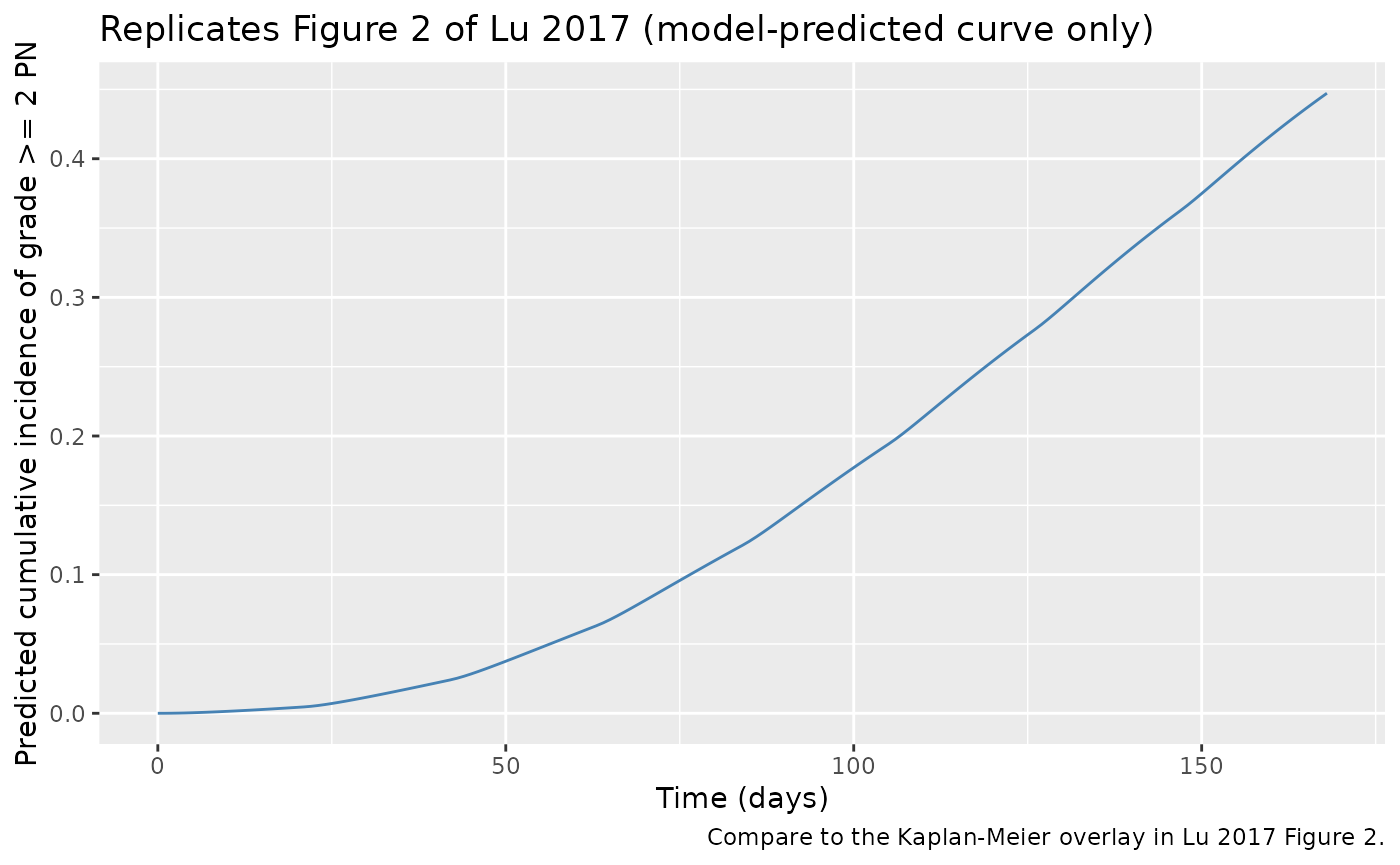
Replicate Figure 4 / Table 2 – dose-response over 6 to 8 cycles
Lu 2017 Figure 4a (nominal doses) and Table 2 quantify the dose-response contrast between pola 1.8 and 2.4 mg/kg q3w over 6 cycles (126 days) and 8 cycles (168 days). The cumulative-incidence trajectories below stratify the virtual cohort by assigned dose level.
km_by_arm <- sim |>
  group_by(time, arm) |>
  summarise(incidence = 1 - mean(surv), .groups = "drop")

ggplot(km_by_arm, aes(time / 24, incidence, colour = arm)) +
  geom_line(linewidth = 0.8) +
  geom_vline(xintercept = c(126, 168), linetype = "dotted", colour = "grey30") +
  labs(x       = "Time (days)",
       y       = "Predicted cumulative incidence of grade >= 2 PN",
       title   = "Replicates Figure 4a of Lu 2017 (nominal-dose dose-response)",
       colour  = "Pola dose",
       caption = "Vertical dotted lines mark the 6-cycle (126 d) and 8-cycle (168 d) endpoints quantified in Table 2.") +
  scale_y_continuous(limits = c(0, NA))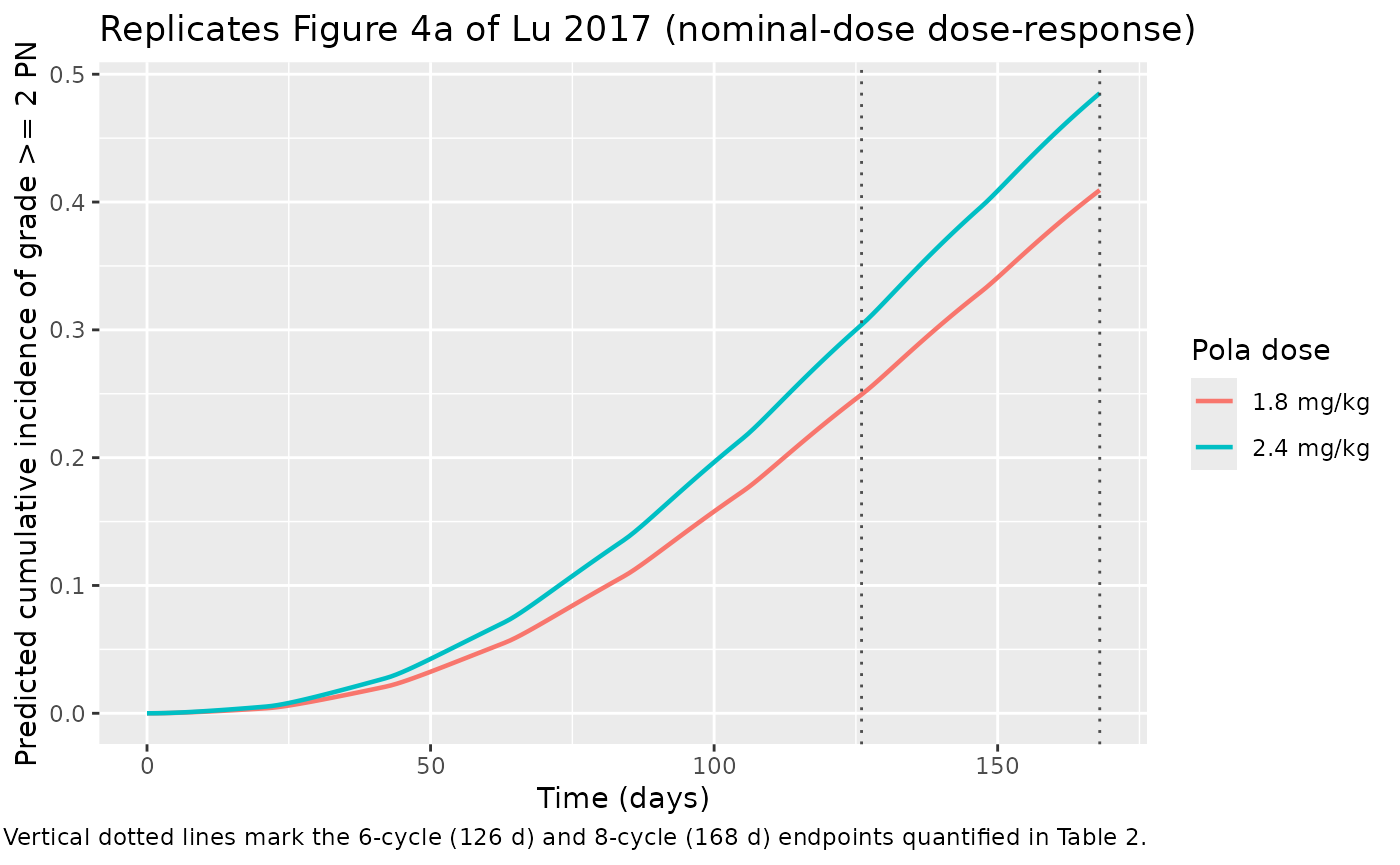
The next chunk extracts the predicted cumulative incidences at 6 and 8 cycles and the per-endpoint risk ratio for 2.4 vs 1.8 mg/kg. Lu 2017 Table 2 reports the following nominal-dose values for comparison:
| Endpoint | 1.8 mg/kg | 2.4 mg/kg | RR (2.4 vs 1.8) |
|---|---|---|---|
| 126 d / 6 cyc | 19.0% (90% CI 13.5-24.7) | 26.6% (90% CI 19.4-33.4) | 1.38 (90% CI 1.30-1.55) |
| 168 d / 8 cyc | 30.7% (90% CI 21.9-38.6) | 40.9% (90% CI 30.9-49.5) | 1.32 (90% CI 1.25-1.47) |
ts_hours <- c(126 * 24, 168 * 24)
tbl <- km_by_arm |>
  filter(time %in% ts_hours) |>
  pivot_wider(names_from = arm, values_from = incidence) |>
  mutate(cycles = ifelse(time == ts_hours[1], "6 cycles (126 d)",
                                                "8 cycles (168 d)"),
         RR_2.4_vs_1.8 = `2.4 mg/kg` / `1.8 mg/kg`) |>
  select(cycles, `1.8 mg/kg`, `2.4 mg/kg`, RR_2.4_vs_1.8)
print(tbl)
#> # A tibble: 2 × 4
#>   cycles           `1.8 mg/kg` `2.4 mg/kg` RR_2.4_vs_1.8
#>   <chr>                  <dbl>       <dbl>         <dbl>
#> 1 6 cycles (126 d)       0.249       0.304          1.22
#> 2 8 cycles (168 d)       0.409       0.485          1.19
The vignette-simulated risk ratios should fall in the same direction as Lu 2017 Table 2 (RR > 1; 2.4 mg/kg confers a higher PN risk than 1.8 mg/kg) and in a comparable magnitude (~1.3-1.4 over 6 to 8 cycles), though absolute incidence values are expected to differ from Table 2 because the model file’s upstream acMMAE PK is taken from the published Lu 2019 integrated 2-analyte popPK (which is more sophisticated than the Lu 2015 ASCPT-poster popPK that the Lu 2017 TTE PD parameters were originally fit against – see Assumptions and deviations below).
Mechanistic sanity checks
The model exposes the instantaneous hazard hazard, the
cumulative hazard cumhaz, and the survival probability
surv = exp(-cumhaz) as derived outputs for direct VPC
simulation. The checks below exercise each mechanistic feature.
1. Hazard rises and falls with the dosing cycle
The base hazard
h_base = beta * (alpha * Ce(t))^beta * t^(beta - 1)
combines a Weibull t^(beta - 1) time scaling (monotone
increasing for beta = 1.37 > 1) with a Ce(t)^beta factor
that tracks the effect-compartment concentration. The hazard therefore
should oscillate within each Q3W dosing cycle (peaking when Ce is
highest, dipping in the trough) while the cycle-by-cycle envelope grows
over time.
sim_ref <- sim |>
  filter(id == 1)
ggplot(sim_ref, aes(time / 24, hazard)) +
  geom_line(colour = "firebrick") +
  geom_vline(xintercept = seq(0, 168, by = 21), linetype = "dotted",
             colour = "grey60") +
  labs(x = "Time (days)", y = "Instantaneous hazard (1/hour)",
       title = "Per-subject hazard trajectory (subject 1)",
       caption = "Vertical lines mark Q3W dose times. Within-cycle oscillation comes from Ce(t); the cycle envelope grows under Weibull beta > 1.")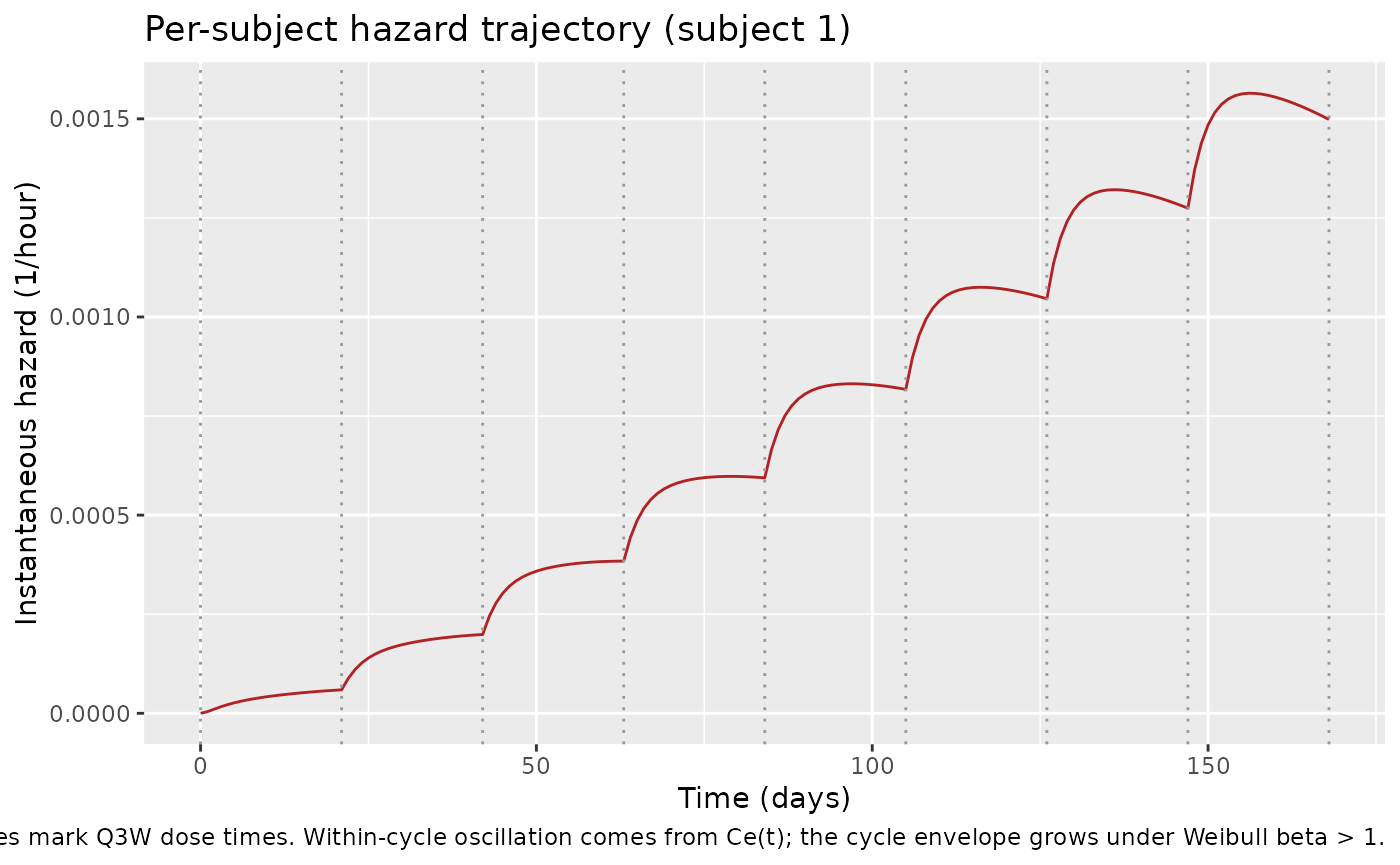
3. Higher body weight increases the hazard (per Lu 2017 Figure 3, theta_bw > 0)
The Figure 3 forest plot reports a median hazard ratio of 1.56 for 100 vs 80 kg, i.e. higher body weight is associated with a higher grade >= 2 PN hazard after adjusting for acMMAE exposure. The check below toggles WT between 60 / 80 / 100 kg in a typical-value (no-eta) simulation and confirms the ordering of cumulative incidence.
m_typ <- rxode2::zeroRe(m)
ev_typ <- function(id, wt) {
  ev <- make_subject(id = id, dose_mg_per_kg = 1.8)
  ev$WT <- wt
  ev$AGE <- 65L; ev$SEXF <- 0L; ev$ALB <- 39
  ev$TUMSZ <- 3000; ev$BLBCELL <- 50
  ev$TUMTP_DLBCL <- 0L; ev$TUMTP_OTHER_NHL <- 0L
  ev$BL_PN_GR1 <- 0L
  ev$PRIOR_RADIATION <- 0L; ev$PRIOR_VINCA <- 0L; ev$PRIOR_PLATIN <- 0L
  ev$CONMED_RITUX <- 1L; ev$LINE_1L <- 0L; ev$RACE_ASIAN <- 0L
  ev$amt[ev$evid == 1L] <- pola_to_mmae_ug(1.8, wt)
  ev$arm <- paste0("WT = ", wt, " kg")
  ev
}
wt_sweep <- bind_rows(ev_typ(1L, 60), ev_typ(2L, 80), ev_typ(3L, 100))
sim_wt   <- rxode2::rxSolve(m_typ, events = wt_sweep, keep = c("arm")) |>
  as.data.frame()
#> ℹ omega/sigma items treated as zero: 'etalcl_time', 'etalcl', 'etalvc', 'etalvp', 'etalq', 'etalvmax'
#> Warning: multi-subject simulation without without 'omega'
incidence_at_168 <- sim_wt |>
  filter(time == max(time)) |>
  mutate(incidence = 1 - surv) |>
  select(arm, incidence)
print(incidence_at_168)
#>           arm incidence
#> 1  WT = 60 kg 0.1770705
#> 2  WT = 80 kg 0.2879818
#> 3 WT = 100 kg 0.4378940
stopifnot(incidence_at_168$incidence[incidence_at_168$arm == "WT = 100 kg"] >
          incidence_at_168$incidence[incidence_at_168$arm == "WT = 80 kg"])
stopifnot(incidence_at_168$incidence[incidence_at_168$arm == "WT = 80 kg"] >
          incidence_at_168$incidence[incidence_at_168$arm == "WT = 60 kg"])
Assumptions and deviations
-
Upstream PK source substitution. The Lu 2017 TTE PD
parameters were fit by NONMEM using empirical-Bayes (EBE) individual PK
parameters from a previously developed Lu 2015 ASCPT-poster popPK model
that is not in the peer-reviewed literature and is not on disk for this
extraction. Per the standing nlmixr2lib policy of reusing a published
same-drug PK as the upstream layer, the model file inlines the acMMAE
side of the peer-reviewed Lu 2019 integrated two-analyte popPK
(
Lu_2019_polatuzumab.R). The Lu 2019 PK is more sophisticated than the Lu 2015 poster popPK – adding a Hill-shaped time-decay on CL_NS, a separate exponential decay on CL_t, Michaelis-Menten elimination, and several covariates not present in the 2015 model – and therefore produces somewhat different acMMAE concentration profiles than were used to fit the Lu 2017 TTE PD parameters. The absolute predicted PN incidences in the Table 2 reproduction above are therefore expected to diverge from Lu 2017 Table 2 values, but the dose-response direction (2.4 mg/kg > 1.8 mg/kg), time trend (incidence increases with cycle count), and risk-ratio magnitude (around 1.3-1.4 between 6 and 8 cycles) should be preserved. -
TTE PD parameters have no IIV. Lu 2017 reports a
single point estimate (with RSE / SE) for each of alpha, beta, k1e, and
the 12 covariate effects, with no omega block on the TTE PD parameters;
the paper’s sequential PK-then-PD fitting strategy and the limited
number of events per patient (one observed PN onset, or right-censoring)
preclude estimating IIV on PD. The model file therefore records the TTE
PD parameters as typical-value-only (no
eta*terms onlalpha_haz,lbeta_haz,lk1e_haz, or any of thee_*_hazcovariate effects). The PK side retains the Lu 2019 acMMAE IIVs. -
CONMED_RITUX double-duty. The Lu 2017 paper’s
rituximabcovariate and the Lu 2019 PK-sideCOMBO_RG(anti-CD20 = rituximab OR obinutuzumab) indicator collapse onto a singleCONMED_RITUXcolumn in the model file. This is exact for the Lu 2017 cohort because no Lu 2017 patient received obinutuzumab combination (the obinutuzumab combinations were added in the later studies GO29365 and GO29044 that motivated the Lu 2019 popPK model but predate the Lu 2017 TTE dataset). Downstream users simulating a Lu 2019-style cohort that includes obinutuzumab patients should setCONMED_RITUX = 1for any anti-CD20 combination (rituximab or obinutuzumab) on the PK side; the Lu 2017 TTE PD layer becomes inexact for obinutuzumab patients but defensible (rituximab and obinutuzumab both deplete B cells). -
Two reference-value conventions on shared
covariates. WT, ALB, and TUMSZ are each used at one reference
value on the PK side (75 kg, 35 g/L, 5000 mm^2 SPD per the Lu 2019
NONMEM control stream) and at a different reference value on the TTE PD
side (80 kg, 39 g/L, 3000 mm^2 per Lu 2017 Eq. 2). These are independent
normalizations of the same physical column and are applied separately in
model(); no value translation is needed on the dataset side. - Virtual cohort covariate distributions. Lu 2017 Supplemental Table S1 tabulates per-patient covariate distributions but the supplement is not on disk; the vignette draws WT, AGE, ALB, TUMSZ, and binary history indicators from defensible distributions anchored at the Figure 3 forest-plot reference values. The qualitative dose-response and covariate-shift checks below should be insensitive to the exact draw.
-
Errata search. A search for corrections / errata to
Lu 2017 (publisher landing page, PMC, Google Scholar
"Lu 2017 polatuzumab vedotin" erratum) returned no results as of 2026-06-24.