Sufentanil (Khaowroongrueng 2024)
Source:vignettes/articles/Khaowroongrueng_2024_sufentanil.Rmd
Khaowroongrueng_2024_sufentanil.RmdModel and source
- Citation: Khaowroongrueng V, Son KH, Lee S-M, Lee J, Park C-G, Lee SI, Shin D, Shin K-H. Population pharmacokinetic modeling of sufentanil in adult Korean patients undergoing cardiopulmonary bypass surgery. CPT Pharmacometrics Syst Pharmacol 2024;13(10):1682-1692. doi:10.1002/psp4.13205.
- Description: Two-compartment IV population PK model for sufentanil in adult Korean patients undergoing cardiac surgery with cardiopulmonary bypass (CPB). First-order elimination, no absorption (IV bolus plus continuous infusion into the central compartment). Two time-varying intra-operative CPB-phase indicators carry the CPB effect: clearance increases 2.80-fold during the CPB and rewarming phases, and the central volume increases 2.74-fold during the CPB phase (hemodilution from the 1700 mL circuit priming volume). The post-CPB phase collapses to the pre-CPB reference. Inter-individual variability was estimated on clearance only (24.2 %CV); Table 2 reports the V1, Q and V2 IIV terms as 0 FIX. Proportional residual error 25.3%. Parameter values from Khaowroongrueng 2024 Table 2.
- Article: CPT Pharmacometrics Syst Pharmacol 2024;13(10):1682-1692
Population
Khaowroongrueng 2024 enrolled 22 adults (>19 years) undergoing cardiac surgery with cardiopulmonary bypass (CPB) support at a single centre in Incheon, South Korea, between May 2021 and June 2022. Table 1 reports a median (range) age of 66 (23-77) years, weight 66.4 (46.7-99.8) kg, height 169.2 (150.1-189.2) cm and body mass index 23.9 (16.0-34.3) kg/m^2, with 14 male and 8 female participants. The predominant procedure was valvuloplasty or valve replacement (13 patients), followed by coronary artery bypass grafting (6), a left ventricular assist device (1) and combination surgery (2). Median (range) CPB duration was 2.3 (1.4-5.6) h within a median total surgical duration of 7.7 (5.3-14.8) h. Patients on renal replacement therapy or taking drugs known to interact with sufentanil were excluded.
Of the 110 samples collected, two participants (12 observations) were excluded for markedly high pre-dose sufentanil concentrations and two further samples were removed as suspected sampling errors, so the final model was fit to 20 participants with 96 observations (Results, “Structural model”). The paper does not re-tabulate demographics for the 20 analysed patients, so the ranges above are the Table 1 values for the 22 enrolled.
Age, height, weight, body mass index, sex, CYP3A4*1G genotype (rs2242480; 13 GG / 6 GA / 3 AA), fluid replacement volumes, and the time-varying laboratory parameters and inflammatory cytokines that changed significantly during CPB (total protein, IL-6, IL-8, TNF-alpha) were all screened. Sex on clearance entered the full model but was dropped at backward elimination, so the CPB phase effects are the only covariates retained in the final model.
The same information is available programmatically via the model’s
population metadata:
pop <- rxode2::rxode(readModelDb("Khaowroongrueng_2024_sufentanil"))$population
#> ℹ parameter labels from comments will be replaced by 'label()'
str(pop[c("species", "n_subjects", "age_median", "weight_median")])
#> List of 4
#>  $ species      : chr "human"
#>  $ n_subjects   : int 20
#>  $ age_median   : chr "66 years"
#>  $ weight_median: chr "66.4 kg"
Source trace
Every ini() entry carries an in-file comment naming its
source location in
inst/modeldb/specificDrugs/Khaowroongrueng_2024_sufentanil.R.
They are collected here for review. All final estimates come from Table
2, “Final model / Estimate” column.
| Equation / parameter | Value | Source location |
|---|---|---|
lcl (CL) |
51.8 L/h (RSE 16.4%) | Table 2 |
lvc (V1) |
72.5 L (RSE 12.1%) | Table 2 |
lq (Q) |
55.2 L/h (RSE 17.2%) | Table 2 |
lvp (V2) |
390 L (RSE 43.8%) | Table 2 |
e_cpb_cl |
2.80 (RSE 14.4%) | Table 2, row “CL CPB&warming” |
e_cpb_vc |
2.74 (RSE 18.5%) | Table 2, row “V1 CPB” |
etalcl |
24.2 %CV -> omega^2 = log(CV^2 + 1) = 0.056921 | Table 2, row “IIV CL (CV, %)”; log-normal IIV per Methods, “Structural model” |
| (no IIV on V1 / Q / V2) | 0 FIX | Table 2, rows “IIV V1 / Q / V2 (CV, %)” |
propSd |
0.253 | Table 2, row “RSV sigma_prop (%)” = 25.3% |
| Two-compartment ODEs, first-order elimination | n/a | Methods, “Structural model”; Results, “Structural model” |
| Multiplicative per-phase covariate form | n/a | Equations 1-4 |
| CL effect spans CPB + warming; V1 effect is CPB only; Q and V2 effects not retained | n/a | Results, “CPB-adjusted model” |
| Post-CPB phase reverts to the pre-CPB reference | n/a | Table 2 retains only CL CPB&warming and
V1 CPB; no COV_post-CPB
|
The paper’s Equations 1-4 give, for the jth model parameter,
pre-CPB:   P_i,j = P_pop,j * exp(eta_i,j) * 1
CPB:       P_i,j = P_pop,j * exp(eta_i,j) * COV_CPB
warming:   P_i,j = P_pop,j * exp(eta_i,j) * COV_warming
post-CPB:  P_i,j = P_pop,j * exp(eta_i,j) * COV_post-CPB
that is, a plain multiplicative fold-change on the typical value
within each phase. Because the phase indicators are binary and mutually
exclusive, the model encodes this as
e_cpb_cl^(CPB_ON + CPB_REWARM) on clearance and
e_cpb_vc^CPB_ON on the central volume, which reproduces the
equations above exactly. Note that the central volume returns to its
baseline at the start of rewarming, while clearance
stays elevated until separation from CPB.
Virtual cohort
Original observed data are not publicly available. The cohort below reproduces the simulation scenario the authors specify in Methods, “Simulations”:
- Cardiac surgery lasting 7.5 h, comprising 1.5 h of CPB and a 1 h warming phase.
- CPB commences 2.5 h after the first sufentanil dose.
- Surgery completes within 2.5 h of CPB weaning.
- Concentration-time profiles simulated for 10 h.
That fixes the phase timeline as pre-CPB [0, 2.5), CPB [2.5, 4.0), rewarming [4.0, 5.0) and post-CPB [5.0, 10].
The recommended regimen from Results, “Simulations” is a 30 ug
loading dose, a 40 ug/h maintenance infusion halted after 6 h, and an
additional 60 ug IV bolus at CPB commencement. Sufentanil was given
intravenously, so every dose goes to the central
compartment.
A second, counterfactual arm holds both phase indicators at 0 throughout. It receives an identical dosing history and exists only to isolate the CPB effect; it is not a scenario the paper reports.
set.seed(20240101)

n_per_arm <- 200L

t_cpb_start <- 2.5
t_rewarm    <- 4.0
t_cpb_end   <- 5.0
t_surg_end  <- 7.5
t_inf_stop  <- 6.0

# Observation grid: a regular grid plus tightly-bracketed times at each phase
# boundary so the discontinuities in V1 and CL can be measured exactly.
eps <- 1e-5
obs_times <- sort(unique(c(
  seq(0, 10, by = 0.05),
  t_surg_end,
  c(t_cpb_start, t_rewarm, t_cpb_end, t_inf_stop) - eps,
  c(t_cpb_start, t_rewarm, t_cpb_end, t_inf_stop)
)))

# Helper: one arm as a self-contained data frame of event records.
# `on_cpb` selects whether the CPB phase indicators are exercised.
# `id_offset` keeps IDs disjoint across arms -- duplicate IDs silently
# collapse into a single subject receiving the summed dose.
make_arm <- function(n, arm, on_cpb, id_offset = 0L) {
  ids <- id_offset + seq_len(n)

  doses <- tidyr::expand_grid(
    id = ids,
    tibble::tibble(
      time = c(0, 0, t_cpb_start),
      amt  = c(30, 40 * t_inf_stop, 60),      # loading bolus, 6 h infusion, CPB bolus
      rate = c(0, 40, 0)                       # 40 ug/h infusion; 0 = bolus
    )
  ) |>
    dplyr::mutate(evid = 1L, cmt = "central")

  obs <- tidyr::expand_grid(id = ids, time = obs_times) |>
    dplyr::mutate(amt = NA_real_, rate = 0, evid = 0L, cmt = "central")

  dplyr::bind_rows(doses, obs) |>
    dplyr::mutate(
      arm        = arm,
      # Time-varying CPB phase indicators, mutually exclusive by construction.
      CPB_ON     = as.integer(on_cpb & time >= t_cpb_start & time < t_rewarm),
      CPB_REWARM = as.integer(on_cpb & time >= t_rewarm    & time < t_cpb_end)
    ) |>
    dplyr::arrange(id, time, dplyr::desc(evid))
}

events <- dplyr::bind_rows(
  make_arm(n_per_arm, arm = "CPB surgery",    on_cpb = TRUE,  id_offset =         0L),
  make_arm(n_per_arm, arm = "No CPB (counterfactual)", on_cpb = FALSE, id_offset = n_per_arm)
) |>
  as.data.frame()

# Disjoint-ID guard, and confirm the indicators never overlap.
# Every id must belong to exactly one arm: a shared id across arms would
# silently merge two subjects into one receiving the summed dose history.
stopifnot(
  all(tapply(events$arm, events$id, dplyr::n_distinct) == 1L),
  all(events$CPB_ON + events$CPB_REWARM <= 1L),
  dplyr::n_distinct(events$id) == 2L * n_per_arm,
  # The counterfactual arm must never switch either indicator on.
  all(events$CPB_ON[events$arm != "CPB surgery"] == 0L),
  all(events$CPB_REWARM[events$arm != "CPB surgery"] == 0L)
)
Simulation
Inter-individual variability sits on clearance only (24.2 %CV); Table
2 reports the V1, Q and V2 IIV terms as 0 FIX, so those
parameters carry no between-subject variability.
mod <- readModelDb("Khaowroongrueng_2024_sufentanil")

sim <- rxode2::rxSolve(mod, events = events, keep = c("arm", "CPB_ON", "CPB_REWARM")) |>
  as.data.frame()
#> ℹ parameter labels from comments will be replaced by 'label()'

# `Cc` is the individual prediction; `sim` additionally carries the
# proportional residual error. Figure 3 of the paper is a mean simulated
# concentration-time profile, and the proportional error is mean-zero, so the
# mean of `Cc` is the right comparator.
dplyr::glimpse(sim[, c("id", "time", "arm", "cl", "vc", "central", "Cc")])
#> Rows: 82,000
#> Columns: 7
#> $ id      <int> 1, 1, 1, 1, 1, 1, 1, 1, 1, 1, 1, 1, 1, 1, 1, 1, 1, 1, 1, 1, 1,…
#> $ time    <dbl> 0.00, 0.05, 0.10, 0.15, 0.20, 0.25, 0.30, 0.35, 0.40, 0.45, 0.…
#> $ arm     <chr> "CPB surgery", "CPB surgery", "CPB surgery", "CPB surgery", "C…
#> $ cl      <dbl> 48.00381, 48.00381, 48.00381, 48.00381, 48.00381, 48.00381, 48…
#> $ vc      <dbl> 72.5, 72.5, 72.5, 72.5, 72.5, 72.5, 72.5, 72.5, 72.5, 72.5, 72…
#> $ central <dbl> 30.00000, 29.87338, 29.76318, 29.66817, 29.58725, 29.51936, 29…
#> $ Cc      <dbl> 0.4137931, 0.4120466, 0.4105266, 0.4092162, 0.4080999, 0.40716…
A deterministic typical-value solve is used for the exact structural
checks below. Rather than zeroRe() (which mutates shared
model state), the etas are supplied as data columns with
omega = NA.
Structural checks against the published covariate model
The per-phase fold-changes are exact multiplicative statements, so
they can be gated exactly rather than eyeballed. In the CPB arm the
typical-value solve must show clearance at 51.8 * 2.80 L/h
throughout CPB and rewarming, and the central volume at
72.5 * 2.74 L during CPB only.
typ_cpb <- sim_typ |> dplyr::filter(arm == "CPB surgery", time > 0)

phase_of <- function(time) {
  dplyr::case_when(
    time <  t_cpb_start ~ "pre-CPB",
    time <  t_rewarm    ~ "CPB",
    time <  t_cpb_end   ~ "rewarming",
    TRUE                ~ "post-CPB"
  )
}

param_by_phase <- typ_cpb |>
  dplyr::mutate(phase = phase_of(time)) |>
  dplyr::group_by(phase) |>
  dplyr::summarise(cl = unique(round(cl, 6)), vc = unique(round(vc, 6)),
                   .groups = "drop") |>
  dplyr::mutate(phase = factor(phase,
    levels = c("pre-CPB", "CPB", "rewarming", "post-CPB"))) |>
  dplyr::arrange(phase)

param_by_phase |>
  dplyr::mutate(
    `CL fold-change` = round(cl / 51.8, 3),
    `V1 fold-change` = round(vc / 72.5, 3)
  ) |>
  dplyr::rename("Phase" = phase, "CL (L/h)" = cl, "V1 (L)" = vc) |>
  knitr::kable(caption = paste(
    "Typical-value CL and V1 by CPB phase. Expected fold-changes:",
    "CL 2.80 during CPB and rewarming, V1 2.74 during CPB only",
    "(Khaowroongrueng 2024 Table 2)."
))| Phase | CL (L/h) | V1 (L) | CL fold-change | V1 fold-change |
|---|---|---|---|---|
| pre-CPB | 51.80 | 72.50 | 1.0 | 1.00 |
| CPB | 145.04 | 198.65 | 2.8 | 2.74 |
| rewarming | 145.04 | 72.50 | 2.8 | 1.00 |
| post-CPB | 51.80 | 72.50 | 1.0 | 1.00 |
expected <- tibble::tibble(
  phase = factor(c("pre-CPB", "CPB", "rewarming", "post-CPB"),
                 levels = c("pre-CPB", "CPB", "rewarming", "post-CPB")),
  cl    = 51.8 * c(1, 2.80, 2.80, 1),
  vc    = 72.5 * c(1, 2.74, 1,    1)
)

stopifnot(
  isTRUE(all.equal(param_by_phase$cl, expected$cl, tolerance = 1e-6)),
  isTRUE(all.equal(param_by_phase$vc, expected$vc, tolerance = 1e-6))
)
The V1 discontinuity is also visible in the concentration itself. No dose is given at the start of rewarming and the amount in the central compartment is continuous there, so the concentration must jump upward by exactly the 2.74-fold V1 ratio as V1 returns to baseline.
before <- typ_cpb |> dplyr::filter(abs(time - (t_rewarm - eps)) < 1e-9)
after  <- typ_cpb |> dplyr::filter(abs(time -  t_rewarm)        < 1e-9)

jump <- tibble::tibble(
  `Quantity`                 = c("central (ug)", "V1 (L)", "Cc (ng/mL)"),
  `Just before rewarming`    = c(before$central, before$vc, before$Cc),
  `At start of rewarming`    = c(after$central,  after$vc,  after$Cc),
  `Ratio (after / before)`   = c(after$central / before$central,
                                after$vc      / before$vc,
                                after$Cc      / before$Cc)
)

knitr::kable(jump, digits = 4, caption = paste(
  "Amount is continuous across the CPB-to-rewarming boundary while V1 reverts,",
  "so Cc rises by exactly the published 2.74-fold V1 ratio."
))| Quantity | Just before rewarming | At start of rewarming | Ratio (after / before) |
|---|---|---|---|
| central (ug) | 57.3494 | 57.3493 | 1.000 |
| V1 (L) | 198.6500 | 72.5000 | 0.365 |
| Cc (ng/mL) | 0.2887 | 0.7910 | 2.740 |
Replicate published figures
# Replicates Figure 3 of Khaowroongrueng 2024: mean simulated
# concentration-time profile for the recommended regimen (30 ug loading dose,
# 40 ug/h maintenance infusion, additional 60 ug IV bolus at CPB initiation),
# with the paper's target-concentration reference lines.
fig3 <- sim |>
  dplyr::filter(!is.na(Cc)) |>
  dplyr::group_by(arm, time) |>
  dplyr::summarise(
    Mean = mean(Cc),
    Q05  = quantile(Cc, 0.05),
    Q95  = quantile(Cc, 0.95),
    .groups = "drop"
  )

ggplot(fig3, aes(time, Mean, colour = arm, fill = arm)) +
  geom_ribbon(aes(ymin = Q05, ymax = Q95), alpha = 0.18, colour = NA) +
  geom_line(linewidth = 0.7) +
  annotate("rect", xmin = 0, xmax = 10, ymin = 0.3, ymax = 0.6,
           alpha = 0.08, fill = "black") +
  geom_hline(yintercept = c(0.3, 0.6), linetype = "dotted") +
  geom_hline(yintercept = 0.15, linetype = "dotted", colour = "red") +
  geom_vline(xintercept = c(t_cpb_start, t_rewarm, t_cpb_end, t_surg_end),
             linetype = "dashed", alpha = 0.35) +
  labs(
    x = "Time (h)", y = "Sufentanil concentration (ng/mL)",
    colour = NULL, fill = NULL,
    title = "Figure 3 - recommended regimen, mean simulated profile",
    caption = paste(
      "Replicates Figure 3 of Khaowroongrueng 2024. Ribbon = 5th-95th",
      "percentile. Dotted black lines: 0.3-0.6 ng/mL target for adequate",
      "anaesthesia. Dotted red line: 0.15 ng/mL end-of-surgery target.",
      "Dashed verticals: CPB start (2.5 h), rewarming (4 h), CPB end (5 h),",
      "end of surgery (7.5 h)."
    )
  ) +
  theme_bw() +
  theme(legend.position = "top", plot.caption = element_text(hjust = 0))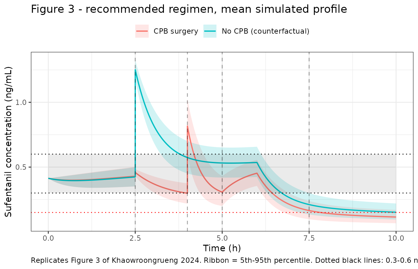
The two CPB effects act in opposite directions at commencement, so the net step is computed rather than asserted. Results states the extra 60 ug bolus was given “to account for the hemodilution effect”, i.e. it is meant to offset the 2.74-fold rise in V1; whether it under- or over-compensates is a quantitative question about this model.
mean_cc <- function(t, arm_name) {
  mean(sim$Cc[sim$arm == arm_name & abs(sim$time - t) < 1e-9], na.rm = TRUE)
}

# Mean central amount just before CPB, used to build the "dilution alone"
# counterfactual: what the concentration would have been at commencement had
# the 60 ug bolus not been given and only the 2.74-fold V1 step applied.
amt_pre  <- mean(sim$central[sim$arm == "CPB surgery" &
                             abs(sim$time - (t_cpb_start - eps)) < 1e-9])
dilution_only <- amt_pre / (72.5 * 2.74)

cc_pre    <- mean_cc(t_cpb_start - eps, "CPB surgery")
cc_onset  <- mean_cc(t_cpb_start,       "CPB surgery")
onset_pct <- 100 * (cc_onset / cc_pre - 1)

onset <- tibble::tibble(
  Quantity = c(
    "CPB arm, just before CPB (2.5 h)",
    "CPB arm, at commencement (2.74-fold V1 step + 60 ug bolus)",
    "Counterfactual: 2.74-fold dilution alone, no bolus",
    "CPB arm, end of CPB (4.0 h, before V1 reverts)",
    "CPB arm, start of rewarming (V1 reverts to baseline)",
    "No-CPB arm, at CPB start (2.5 h)",
    "No-CPB arm, at CPB end (5.0 h)"
  ),
  `Mean Cc (ng/mL)` = c(
    cc_pre, cc_onset, dilution_only,
    mean_cc(t_rewarm - eps, "CPB surgery"),
    mean_cc(t_rewarm,       "CPB surgery"),
    mean_cc(t_cpb_start,    "No CPB (counterfactual)"),
    mean_cc(t_cpb_end,      "No CPB (counterfactual)")
  )
)

knitr::kable(onset, digits = 3, caption = paste(
  "Mean simulated concentrations across the bypass window. The",
  "dilution-alone row is a counterfactual, not a simulated arm: it applies",
  "the 2.74-fold V1 step to the observed pre-CPB amount without the 60 ug",
  "bolus."
))| Quantity | Mean Cc (ng/mL) |
|---|---|
| CPB arm, just before CPB (2.5 h) | 0.430 |
| CPB arm, at commencement (2.74-fold V1 step + 60 ug bolus) | 0.459 |
| Counterfactual: 2.74-fold dilution alone, no bolus | 0.157 |
| CPB arm, end of CPB (4.0 h, before V1 reverts) | 0.298 |
| CPB arm, start of rewarming (V1 reverts to baseline) | 0.817 |
| No-CPB arm, at CPB start (2.5 h) | 1.252 |
| No-CPB arm, at CPB end (5.0 h) | 0.532 |
# When the counterfactual arm's mean profile drops back below the 0.6 ng/mL
# anaesthesia ceiling, expressed as a fraction of the way through the bypass
# window. Quoted in the narrative below.
noc <- sim |>
  dplyr::filter(arm == "No CPB (counterfactual)", !is.na(Cc),
                time >= t_cpb_start, time <= t_cpb_end) |>
  dplyr::group_by(time) |>
  dplyr::summarise(mean_cc = mean(Cc), .groups = "drop")
t_cross  <- min(noc$time[noc$mean_cc < 0.6])
frac_win <- (t_cross - t_cpb_start) / (t_cpb_end - t_cpb_start)

# Monte-Carlo precision of the mean profile at this cohort size: the largest
# standard error of the mean across the observation grid, as a percentage of the
# mean at that time. Quoted in "Assumptions and deviations" below.
sem_max <- sim |>
  dplyr::filter(arm == "CPB surgery", !is.na(Cc), time > 0) |>
  dplyr::group_by(time) |>
  dplyr::summarise(sem_pct = 100 * sd(Cc) / sqrt(dplyr::n()) / mean(Cc),
                   .groups = "drop") |>
  dplyr::pull(sem_pct) |>
  max()

stopifnot(
  # The bolus more than offsets hemodilution: the net step at commencement is UP.
  onset_pct > 0,
  # Dilution alone would have cut the concentration by more than half.
  dilution_only < 0.5 * cc_pre,
  # Clearance is 2.80-fold higher through CPB, so the decline is faster: the
  # concentration must fall below its pre-CPB level by the end of the phase.
  mean_cc(t_rewarm - eps, "CPB surgery") < cc_pre,
  # The counterfactual arm never drops below the CPB arm during the window.
  mean_cc(t_cpb_start, "No CPB (counterfactual)") > cc_onset
)
The 60 ug bolus therefore over-compensates: the mean concentration steps up by 6.8% at commencement (0.430 to 0.459 ng/mL), whereas the 2.74-fold dilution acting alone would have taken it to 0.157 ng/mL. What the CPB arm does show is the second effect, the 2.80-fold clearance increase: the concentration falls from 0.459 to 0.298 ng/mL over the 1.5 h bypass phase, well below its pre-CPB level. V1 then reverts at the start of rewarming and the concentration jumps to 0.817 ng/mL, the highest mean in this arm – which is why the NCA table above reports Tmax at 4.0 h rather than at a dosing time.
The counterfactual no-CPB arm, receiving an identical dosing history, runs above the CPB arm throughout the bypass window (1.252 ng/mL at CPB start, declining to 0.532 ng/mL by CPB end) – it starts well above the 0.6 ng/mL anaesthesia ceiling and does not drop back into the 0.3-0.6 band until 3.80 h, about 52% of the way through the window. This is the model-side counterpart of the paper’s Discussion claim that “using pharmacokinetic parameters obtained from patients undergoing general anesthesia for sufentanil TCI during cardiac surgery with CPB is not suitable”: ignoring the phase effects overstates exposure during bypass.
PKNCA validation
sim_nca <- sim |>
  dplyr::filter(!is.na(Cc)) |>
  dplyr::select(id, time, Cc, arm)

# Guarantee a time = 0 record per subject to anchor AUC from 0.
sim_nca <- dplyr::bind_rows(
  sim_nca,
  sim_nca |> dplyr::distinct(id, arm) |> dplyr::mutate(time = 0, Cc = 0)
) |>
  dplyr::distinct(id, arm, time, .keep_all = TRUE) |>
  dplyr::arrange(id, arm, time)

conc_obj <- PKNCA::PKNCAconc(sim_nca, Cc ~ time | arm + id)

# Doses: the loading bolus, the 6 h infusion, and the CPB bolus. The loading
# bolus and the start of the infusion coincide at t = 0, and PKNCA requires a
# single dose record per subject and time, so the two coincident events are
# pooled into one record (270 ug delivered from t = 0, the longer of the two
# durations). None of the NCA parameters requested below is dose-normalised, so
# the pooling does not affect any reported value -- the dose object here only
# supplies the dosing times that anchor the interval.
dose_df <- events |>
  dplyr::filter(evid == 1) |>
  dplyr::mutate(duration = ifelse(rate > 0, amt / rate, 0)) |>
  dplyr::group_by(id, arm, time) |>
  dplyr::summarise(amt = sum(amt), duration = max(duration), .groups = "drop")

stopifnot(!anyDuplicated(dose_df[, c("id", "arm", "time")]))

dose_obj <- PKNCA::PKNCAdose(dose_df, amt ~ time | arm + id, duration = "duration")

# The surgical window [0, 7.5 h] is the interval the paper's targets refer to.
intervals <- data.frame(
  start   = 0,
  end     = t_surg_end,
  cmax    = TRUE,
  tmax    = TRUE,
  auclast = TRUE,
  cav     = TRUE
)

nca_res <- PKNCA::pk.nca(PKNCA::PKNCAdata(conc_obj, dose_obj, intervals = intervals))

nca_summary <- as.data.frame(nca_res) |>
  dplyr::group_by(arm, PPTESTCD) |>
  dplyr::summarise(Median = median(PPORRES), .groups = "drop") |>
  tidyr::pivot_wider(names_from = PPTESTCD, values_from = Median)

nca_summary |>
  dplyr::rename(
    "Arm"                     = arm,
    "Cmax (ng/mL)"            = cmax,
    "Tmax (h)"                = tmax,
    "AUC0-7.5h (ng*h/mL)"     = auclast,
    "Cav 0-7.5h (ng/mL)"      = cav
  ) |>
  knitr::kable(digits = 3, caption = paste(
    "Median simulated NCA parameters over the 7.5 h surgical window.",
    "Khaowroongrueng 2024 reports no NCA table, so these are not a",
    "reproduction of published values."
))| Arm | AUC0-7.5h (ng*h/mL) | Cav 0-7.5h (ng/mL) | Cmax (ng/mL) | Tmax (h) |
|---|---|---|---|---|
| CPB surgery | 2.804 | 0.374 | 0.820 | 4.0 |
| No CPB (counterfactual) | 3.787 | 0.505 | 1.257 | 2.5 |
Comparison against published target concentrations
Khaowroongrueng 2024 reports no NCA table, so there are no published
Cmax / AUC / half-life values to compare against and
ncaComparisonTable() is not applicable. What the paper does
report quantitatively about its simulation are the target concentrations
that drove the dose recommendation (Methods, “Simulations”; Results,
“Simulations”; Figure 3). Those are compared below.
cc_at <- function(t, arm_name = "CPB surgery") {
  sim |>
    dplyr::filter(arm == arm_name, abs(time - t) < 1e-9, !is.na(Cc)) |>
    dplyr::pull(Cc) |>
    mean()
}

# Mean concentration over the maintenance window (post-loading, pre-CPB and
# the post-CPB remainder of surgery), where the 0.3-0.6 ng/mL anaesthesia
# target applies.
maint <- sim |>
  dplyr::filter(arm == "CPB surgery", !is.na(Cc),
                time >= 0.5, time <= t_surg_end) |>
  dplyr::pull(Cc)

comparison <- tibble::tribble(
  ~Milestone,                                  ~`Paper's target`,        ~Simulated,
  "Just before CPB (2.5 h)",                   "at least 0.5-0.7 ng/mL", cc_at(t_cpb_start - eps),
  "During CPB (3.0 h)",                        "(not targeted)",         cc_at(3.0),
  "End of surgery (7.5 h)",                    "approx. 0.15 ng/mL",     cc_at(t_surg_end),
  "Mean over surgery (0.5-7.5 h)",             "0.3-0.6 ng/mL",          mean(maint)
)

comparison |>
  dplyr::mutate(Simulated = round(Simulated, 3)) |>
  knitr::kable(caption = paste(
    "Simulated mean concentrations at the milestones",
    "Khaowroongrueng 2024 used to justify the recommended regimen",
    "(Methods and Results, 'Simulations'; Figure 3)."
))| Milestone | Paper’s target | Simulated |
|---|---|---|
| Just before CPB (2.5 h) | at least 0.5-0.7 ng/mL | 0.430 |
| During CPB (3.0 h) | (not targeted) | 0.375 |
| End of surgery (7.5 h) | approx. 0.15 ng/mL | 0.165 |
| Mean over surgery (0.5-7.5 h) | 0.3-0.6 ng/mL | 0.373 |
# The end-of-surgery target is the paper's most specific quantitative claim
# about this regimen: Results recommends the infusion "be halted after 6 h,
# aligning with a target concentration of 0.15 ng/mL at the conclusion of the
# surgery", on the assumption that surgery concludes within 1.5 h of cessation.
stopifnot(
  cc_at(t_surg_end) > 0.12, cc_at(t_surg_end) < 0.19,
  # Mean exposure across the surgical window sits inside the anaesthesia band.
  mean(maint) > 0.3, mean(maint) < 0.6
)
The end-of-surgery concentration (0.165 ng/mL) and the mean over the surgical window (0.373 ng/mL) both land where the paper says they should. The pre-CPB value does not: at 0.430 ng/mL it sits below the “at least 0.5-0.7 ng/mL” figure quoted in Methods, “Simulations”.
Methods ties that figure to three quantities jointly: “doses of sufentanil were varied to propose a loading dose (25-40 ug) and an additional IV bolus dose (50-80 ug) corresponding to a target concentration of at least 0.5-0.7 ng/mL for pre-CPB control, and an infusion rate (30-45 ug/h) corresponding to a target concentration of 0.3-0.6 ng/mL for adequate anesthesia”. The band itself is carried over from the literature (the paper’s reference 25, Hudson et al.), not estimated here. The sweep below therefore spans the full grid the paper explored – all three ranges, not just the two bolus doses – so that the question “is the band reachable anywhere in the explored space?” is actually tested rather than assumed.
sweep_grid <- tidyr::expand_grid(loading  = c(25, 30, 40),
                                 bolus    = c(50, 60, 80),
                                 infusion = c(30, 40, 45)) |>
  dplyr::mutate(i = dplyr::row_number(),
                arm = paste0(loading, " / ", bolus, " / ", infusion))

ev_sweep <- lapply(seq_len(nrow(sweep_grid)), function(k) {
  g <- sweep_grid[k, ]
  make_arm(1L, arm = g$arm, on_cpb = TRUE, id_offset = 1000L * g$i) |>
    dplyr::mutate(
      # `amt` is computed before `rate` is overwritten, so the rate == 0 /
      # rate > 0 tests below still see the original infusion flag.
      amt = dplyr::case_when(
        # The loading bolus is the t = 0 dose record with rate == 0.
        evid == 1L & time == 0 & rate == 0 ~ g$loading,
        # The infusion is the t = 0 dose record with rate > 0; its total amount
        # must track the rate so the duration stays at t_inf_stop.
        evid == 1L & time == 0 & rate >  0 ~ g$infusion * t_inf_stop,
        # The additional bolus is the dose record at CPB commencement.
        evid == 1L & time == t_cpb_start   ~ g$bolus,
        TRUE                               ~ amt
      ),
      rate = ifelse(evid == 1L & time == 0 & rate > 0, g$infusion, rate)
    )
}) |>
  dplyr::bind_rows() |>
  dplyr::mutate(etalcl = 0) |>
  as.data.frame()

sweep_sim <- rxode2::rxSolve(mod, events = ev_sweep, omega = NA, keep = "arm") |>
  as.data.frame()
#> Warning: multi-subject simulation without without 'omega'

sweep <- sweep_sim |>
  dplyr::filter(abs(time - (t_cpb_start - eps)) < 1e-9 |
                abs(time -  t_cpb_start)        < 1e-9) |>
  dplyr::mutate(when = ifelse(time < t_cpb_start, "before", "after")) |>
  dplyr::select(arm, when, Cc) |>
  tidyr::pivot_wider(names_from = when, values_from = Cc) |>
  dplyr::left_join(sweep_grid, by = "arm") |>
  dplyr::arrange(infusion, bolus, loading)

# Summary quantities the narrative below quotes, so the prose cannot drift from
# the table.
sweep_max_before <- max(sweep$before)
sweep_n_before   <- sum(sweep$before >= 0.5)
sweep_n_after    <- sum(sweep$after  >= 0.5)
# Spread attributable to the loading dose alone, holding bolus and infusion at
# the recommended 60 ug / 40 ug/h.
sweep_rec <- sweep |> dplyr::filter(bolus == 60, infusion == 40)

sweep |>
  dplyr::transmute(
    `Loading (ug)`                    = loading,
    `CPB bolus (ug)`                  = bolus,
    `Infusion (ug/h)`                 = infusion,
    `Cc just before CPB (ng/mL)`      = round(before, 3),
    `Cc just after CPB bolus (ng/mL)` = round(after, 3),
    `Either >= 0.5 ng/mL`             = ifelse(pmax(before, after) >= 0.5,
                                               "yes", "no")
  ) |>
  knitr::kable(caption = paste(
    "Typical-value concentrations at CPB commencement across the full",
    "loading-dose, additional-bolus and infusion-rate grid Khaowroongrueng",
    "2024 explored (Methods, 'Simulations')."
))| Loading (ug) | CPB bolus (ug) | Infusion (ug/h) | Cc just before CPB (ng/mL) | Cc just after CPB bolus (ng/mL) | Either >= 0.5 ng/mL |
|---|---|---|---|---|---|
| 25 | 50 | 30 | 0.319 | 0.368 | no |
| 30 | 50 | 30 | 0.323 | 0.370 | no |
| 40 | 50 | 30 | 0.332 | 0.373 | no |
| 25 | 60 | 30 | 0.319 | 0.418 | no |
| 30 | 60 | 30 | 0.323 | 0.420 | no |
| 40 | 60 | 30 | 0.332 | 0.423 | no |
| 25 | 80 | 30 | 0.319 | 0.519 | yes |
| 30 | 80 | 30 | 0.323 | 0.521 | yes |
| 40 | 80 | 30 | 0.332 | 0.524 | yes |
| 25 | 50 | 40 | 0.417 | 0.404 | no |
| 30 | 50 | 40 | 0.422 | 0.406 | no |
| 40 | 50 | 40 | 0.430 | 0.409 | no |
| 25 | 60 | 40 | 0.417 | 0.454 | no |
| 30 | 60 | 40 | 0.422 | 0.456 | no |
| 40 | 60 | 40 | 0.430 | 0.459 | no |
| 25 | 80 | 40 | 0.417 | 0.555 | yes |
| 30 | 80 | 40 | 0.422 | 0.557 | yes |
| 40 | 80 | 40 | 0.430 | 0.560 | yes |
| 25 | 50 | 45 | 0.467 | 0.422 | no |
| 30 | 50 | 45 | 0.471 | 0.424 | no |
| 40 | 50 | 45 | 0.480 | 0.427 | no |
| 25 | 60 | 45 | 0.467 | 0.472 | no |
| 30 | 60 | 45 | 0.471 | 0.474 | no |
| 40 | 60 | 45 | 0.480 | 0.477 | no |
| 25 | 80 | 45 | 0.467 | 0.573 | yes |
| 30 | 80 | 45 | 0.471 | 0.575 | yes |
| 40 | 80 | 45 | 0.480 | 0.578 | yes |
stopifnot(
  # The claim in the narrative: the pre-CPB band is not reached anywhere in the
  # explored grid before the additional bolus is given.
  sweep_n_before == 0L,
  # It IS reached post-bolus somewhere in the grid.
  sweep_n_after > 0L
)
The sweep shows the pre-CPB concentration is almost insensitive to
the loading dose: by 2.5 h the loading bolus has largely distributed and
cleared (V2 = 390 L, CL = 51.8 L/h), so the level is set mostly by the
infusion, which has not yet reached steady state (at the recommended 40
ug/h the asymptote is 40 / 51.8 = 0.772 ng/mL). Holding the
bolus and infusion at the recommended 60 ug and 40 ug/h, the entire
25-40 ug loading range moves the pre-CPB concentration only from 0.417
to 0.430 ng/mL. It is the additional bolus at CPB
commencement that lifts the concentration into the 0.5-0.7
band, and only at the top of the explored 50-80 ug range – the
recommended 60 ug bolus gives 0.456 ng/mL immediately after dosing.
So the recommended regimen does not attain the pre-CPB band under this model, and no combination anywhere in the paper’s explored grid attains it before CPB: across all 27 loading / bolus / infusion combinations the highest pre-CPB concentration is 0.480 ng/mL, reached at the top of the loading and infusion ranges (40 ug loading, 45 ug/h infusion – the additional bolus is given at CPB commencement and so cannot affect the pre-CPB value), still short of 0.5. Post-bolus the band is attainable, in 9 of 27 combinations. Two readings are consistent with the paper: either the 0.5-0.7 ng/mL criterion was applied to the post-bolus concentration at CPB initiation, or the recommendation deliberately trades it off, as Results implies by choosing 30 ug “considering the target concentrations at various CPB phases”. The paper does not tabulate its own simulated concentrations, and Figure 3 is a raster image, so this cannot be settled from the available sources. It is recorded as an open discrepancy rather than resolved by adjusting any parameter.
Assumptions and deviations
- No supplementary material available. Tables S1-S3 and Figures S1-S3 were not available when this model was built. Every final parameter value is in main-text Table 2, so nothing in the model file depends on the supplement. The supplement carries the model-development trail (Table S1), the clinical laboratory / cytokine data (Table S2) and a literature comparison of Vd and Vdss (Table S3) – none of which enters the model.
-
Post-CPB phase collapses to the pre-CPB reference.
Equation 4 admits a distinct
COV_post-CPBmultiplier, but Table 2 retains onlyCL CPB&warmingandV1 CPB, so no post-CPB effect was carried into the final model. The model therefore has noCPB_POSTindicator. -
CPB phase decomposed into two binary indicators.
The paper stores the phase as a single 0/1/2/3 column. Per the standing
convention of decomposing categorical covariates rather than testing
levels inside
model(), this is encoded as the canonicalCPB_ON(phase 1) andCPB_REWARM(phase 2), both newly registered ininst/references/covariate-columns.mdalongside this extraction. The clearance effect uses the sum of the two indicators because the paper estimated a single typical value spanning both windows. -
IIV variance scale. Table 2 reports IIV as %CV and
Methods states a log-normal IIV distribution, so
omega^2 = log(CV^2 + 1) = 0.056921for the 24.2 %CV clearance term. Under the alternative NONMEM convention (omega^2 = CV^2) the variance would be 0.058564; the two differ by 3% in variance and are indistinguishable at the reported 3 significant figures. -
No IIV on V1, Q or V2. Table 2 reports these as
0 FIX, so noetalvc/etalq/etalvpterms are included. The Discussion attributes this to the small sample size limiting IIV estimation. - No IIV on the CPB effects. The paper estimates the phase fold-changes as typical values only.
-
Units. Doses are in ug and volumes in L, so
Cc = central / vcis in ug/L, which is identically ng/mL – the paper’s reporting unit. No scaling factor is needed.checkModelConventions()emits an informational note that the dosing prefix (ug) and the concentration numerator (ng) differ in magnitude; that heuristic does not account for the L-versus-mL denominator, and the relationship is exact here. -
Time-varying V1 produces a discontinuous
concentration. The amount in the central compartment is
continuous across a phase boundary while V1 steps, so
Ccjumps. This is the standard consequence of a time-varying volume in a NONMEM ADVAN3/TRANS4-style parameterisation and reproduces the paper’s Equations 1-4 faithfully; it is not a physiological claim about instantaneous redistribution. - Simulation scenario, not observed data. The observed concentrations are not public. The virtual cohort follows the phase timeline and dosing the authors specify for their own simulation (Methods, “Simulations”), using 200 subjects per arm rather than the paper’s 1000 replicates. With IIV on clearance only (24.2 %CV), the Monte-Carlo standard error of the mean profile at 200 per arm peaks at 1.97% of the mean across the observation grid, so the mean profile the figure and tables report is well determined at this cohort size.
- OPEN DISCREPANCY – the pre-CPB “0.5-0.7 ng/mL” target is not attained. The simulated mean concentration just before CPB under the recommended regimen is 0.430 ng/mL (typical value 0.422), against the “at least 0.5-0.7 ng/mL for pre-CPB control” quoted in Methods, “Simulations”. The dose sweep above shows this is not a loading-dose effect: holding the bolus and infusion at their recommended values, the paper’s entire 25-40 ug loading range moves the pre-CPB concentration only from 0.417 to 0.430 ng/mL, because by 2.5 h the bolus has distributed into the 390 L peripheral compartment and been cleared at 51.8 L/h, leaving the not-yet steady-state infusion to set the level. Sweeping the paper’s full three-way grid (loading, additional bolus and infusion rate) does not close the gap either: the highest pre-CPB concentration anywhere in the 27 combinations is 0.480 ng/mL. Only the additional bolus at CPB commencement reaches the band, and only at the top of its explored 50-80 ug range. The paper does not tabulate its simulated concentrations and Figure 3 is a raster image, so this cannot be settled from the available sources. No parameter was adjusted to close the gap; every value remains as published in Table 2. The two structural gates that are exactly checkable (the 2.80-fold CL and 2.74-fold V1 changes) match to 1e-6, and the paper’s two specific claims about the recommended regimen (0.15 ng/mL at end of surgery, the 0.3-0.6 ng/mL anaesthesia band) are both reproduced, which localises the discrepancy to the dose-selection narrative rather than to the PK model.
- The counterfactual no-CPB arm is not a published scenario. It is included only to isolate the CPB effect and to give the fold-change gates a paired reference.
- Weight and other demographics are not in the model. No allometric or demographic covariate was retained, so the virtual cohort carries no weight column; the loading dose is the paper’s recommended flat 30 ug rather than a per-kg dose.
-
half.lifeis not reported. Over the 7.5 h surgical window the profile never reaches a clean terminal phase (the infusion stops at 6 h), so a half-life estimate would describe distribution rather than terminal elimination and is omitted rather than reported misleadingly.