Sulbactam-durlobactam (Cammarata 2024)

Model and source

• Citation: Cammarata AP, Safir MC, Trang M, Larson KB, O’Donnell JP, Bhavnani SM, Rubino CM. Population pharmacokinetic analyses for sulbactam-durlobactam using Phase 1, 2, and 3 data. Antimicrob Agents Chemother. 2024;69(1):e00485-24. doi:10.1128/aac.00485-24. Plasma model parameters from Table 1, hemodialysis sub-model parameters from Table S4, and epithelial lining fluid sub-model parameters from Table S6 of the supplement.

• Article: https://doi.org/10.1128/aac.00485-24 (open access, CC BY 4.0)

• Supplement (Tables S1-S13, Figures S1-S19): aac.00485-24-s0001.pdf, linked from the article page

Sulbactam-durlobactam (XACDURO) is a beta-lactam / beta-lactamase-inhibitor combination approved in the United States for hospital-acquired and ventilator-associated bacterial pneumonia caused by susceptible isolates of the Acinetobacter baumannii-calcoaceticus complex. Durlobactam (formerly ETX2514) inhibits Class A, C, and D beta-lactamases and restores sulbactam activity against multidrug-resistant A. baumannii.

Structure

Both analytes are two-compartment with linear, first-order elimination, and the two subsystems were fitted simultaneously as a single four-compartment model (NONMEM compartments 1-2 for durlobactam, 3-4 for sulbactam). In the packaged file durlobactam carries the unsuffixed canonical names (central, peripheral1, lcl, lvc, …) and sulbactam carries the registered sibling-drug suffix _sbt.

Total clearance of each drug is the sum of a renal and a non-renal arm:

$$\mathrm{CL_R} = \mathrm{CL}\cdot \mathrm{FE}\cdot\left(\frac{\mathrm{CLcr}}{100}\right)^{\theta_{\mathrm{CLcr}}}, \qquad \mathrm{CL_{NR}} = \mathrm{CL}\cdot(1-\mathrm{FE})$$

$$\mathrm{CL_T} = (\mathrm{CL_R}+\mathrm{CL_{NR}}) \cdot\left(\frac{\mathrm{WT}}{75}\right)^{\theta_{\mathrm{WT}}} \cdot\prod_k \left(1+\theta_k\,X_k\right)\cdot e^{\eta_{\mathrm{CL}}} \cdot \mathrm{HDEFFECT}^{\,\mathrm{HD}}$$

where $X_k$ are the proportional-shift covariates (East Asian region, infection type, and the CLcr < 30 mL/min/1.73 m^2 indicator). Central volume takes the same shape without the renal split and without the hemodialysis term. Only CLcr and body weight enter as power functions; every other covariate is a proportional shift, exactly as stated in the paper’s Results.

The paper’s two sub-models are integrated into the same packaged model:

• the hemodialysis sub-model (Table S4) contributes the $\mathrm{HDEFFECT}^{\,\mathrm{HD}}$ factor above, gated by the time-varying RRT_HEMODIAL_ACTIVE column so that clearance reduces exactly to the plasma value between sessions and in every non-dialysed subject;
• the epithelial lining fluid sub-model (Table S6) contributes the algebraic observables Celf and Celf_sbt, instantaneous ratios of the corresponding plasma concentrations.

Both sub-models were fitted with every plasma term fixed to its Table 1 population mean, so their estimated terms compose directly onto the plasma model without any re-estimation.

mod <- readModelDb("Cammarata_2024_sulbactam_durlobactam")

Population

The plasma model was fitted to 373 subjects contributing 5,188 plasma concentrations pooled from eight studies: six Phase 1 studies (a single/multiple ascending dose study, an ELF penetration study, a renal impairment study, a mass balance study, a thorough-QT study, and a study in Chinese subjects), one Phase 2 study in complicated urinary tract infection and acute pyelonephritis (CS2514-2017-0003), and one Phase 3 study in A. baumannii-calcoaceticus complex infections (CS2514-2017-0004). 3,494 concentrations came from durlobactam (373 subjects) and 1,944 from sulbactam (264 subjects).

Baseline demographics (Table S3, pooled column): median age 46 years (18-91), median weight 75 kg (35.8-150), median BSA-normalized Cockcroft-Gault creatinine clearance 91.5 mL/min/1.73 m^2 (5.61-364), 37.5% female, 65.4% White / 16.1% Asian / 13.1% Black, and 12.1% enrolled in the East Asian region (China, Taiwan, or South Korea). Infection-type counts among the 162 Phase 2 and Phase 3 patients (Table S12): 35 cUTI, 17 acute pyelonephritis, 38 HABP, 56 VABP, and 16 bacteremia. Approximately 14% of post-dose samples were below the limit of quantitation, driven by the short half-lives and the extended Phase 1 sampling schemes: fewer than 1% of BLQ samples fell within the first 12 hours post-dose while 69% fell at 48 hours or later.

The hemodialysis sub-model used 202 Period 2 records from six end-stage renal disease subjects in Cohort 5 of CS2514-2017-0002; the ELF sub-model used 60 ELF records (one sample per analyte per subject) from 30 healthy subjects in CS2514-2017-0001.

The same information is available programmatically:

str(readModelDb("Cammarata_2024_sulbactam_durlobactam")()$population, max.level = 1)
#> List of 16
#>  $ species         : chr "human"
#>  $ n_subjects      : int 373
#>  $ n_studies       : int 8
#>  $ n_concentrations: int 5188
#>  $ age_range       : chr "18-91 years"
#>  $ age_median      : chr "46 years"
#>  $ weight_range    : chr "35.8-150 kg"
#>  $ weight_median   : chr "75 kg"
#>  $ sex_female_pct  : num 37.5
#>  $ race_ethnicity  : Named num [1:5] 65.4 13.1 16.1 1.88 3.49
#>   ..- attr(*, "names")= chr [1:5] "White" "Black" "Asian" "American Indian/Alaska Native" ...
#>  $ disease_state   : chr "Pooled healthy adults (six Phase 1 studies including a dedicated renal-impairment study spanning normal renal f"| __truncated__
#>  $ dose_range      : chr "Durlobactam single doses 0.25-8 g and 0.25-2 g q6h; combination dosing 0.5 g or 1 g sulbactam with 0.5 g or 1 g"| __truncated__
#>  $ regions         : chr "United States and other non-East-Asian sites; China (Studies ZL-2402-001 and part of CS2514-2017-0004), Taiwan,"| __truncated__
#>  $ renal_function  : chr "Baseline BSA-normalized Cockcroft-Gault CLcr 5.61-364 mL/min/1.73 m^2 (pooled median 91.5). The renal-impairmen"| __truncated__
#>  $ bmi_range       : chr "11-52.1 kg/m^2 (pooled median 25.7)"
#>  $ notes           : chr "Baseline demographics from Cammarata 2024 Table S3 (pooled dataset, n = 373). 432 subjects and 8,100 plasma con"| __truncated__

Source trace

Every ini() entry carries an in-file comment naming its source location. The table below collects them.

Equation / parameter	Value	Source location
lcl (durlobactam CL)	9.33 L/h	Table 1, Durlobactam, CL
e_crcl_cl_renal	0.875	Table 1, Durlobactam, CL R, CLcr power
lvc (durlobactam Vc)	12.5 L	Table 1, Durlobactam, Vc
lq (durlobactam Q)	4.43 L/h	Table 1, Durlobactam, Q
lvp (durlobactam Vp)	5.83 L	Table 1, Durlobactam, Vp
f_renal (durlobactam FE)	0.479 (FIXED)	Table 1, Durlobactam, FE (%); Results, model-development paragraph 1
e_region_eastasia_cl	-0.199	Table 1, Durlobactam, CLEASIAFL1
e_wt_cl	0.646	Table 1, Durlobactam, CLWTKG1
e_habp_vabp_vc	1.52	Table 1, Durlobactam, V1INFTYPN1&2 (HABP and VABP)
e_cuti_vc	0.343	Table 1, Durlobactam, V1INFTYPN3 (cUTI)
e_bacteremia_vc	3.32	Table 1, Durlobactam, V1INFTYPN4 (bacteremia)
e_wt_vc	0.521	Table 1, Durlobactam, V1WTKG1
e_region_eastasia_vc	-0.263	Table 1, Durlobactam, V1EASIAFL1
e_renalimp_sev_cl	-0.58	Table 1, Durlobactam, BCLCRNLT30
etalcl, etalvc, covariance	0.0778, 0.0757, 0.0494	Table 1, Durlobactam, omega^2 CL, omega^2 Vc, Covariance
etalvp	0.0773	Table 1, Durlobactam, omega^2 Vp
propSdPhase1, addSdPhase1	sqrt(0.019), sqrt(0.00136)	Table 1, Durlobactam, sigma^2 plasma, Proportional / Additive Phase 1
propSdPhase2, propSdPhase3	sqrt(0.0794), sqrt(0.203)	Table 1, Durlobactam, sigma^2 plasma, Proportional Phase 2 / Phase 3
lcl_sbt (sulbactam CL)	13.5 L/h	Table 1, Sulbactam, CL
e_crcl_cl_renal_sbt	1.14	Table 1, Sulbactam, CL R, CLcr power
lvc_sbt, lq_sbt, lvp_sbt	12 L, 7.88 L/h, 6.99 L	Table 1, Sulbactam, Vc / Q / Vp
f_renal_sbt (sulbactam FE)	0.479 (FIXED)	Table 1, Sulbactam, FE (%)
e_habp_cl_sbt … e_ap_cl_sbt	-0.424, -0.298, -0.157, -0.444, -0.382	Table 1, Sulbactam, CLINFTYPN1-CLINFTYPN5
e_wt_cl_sbt	1.01	Table 1, Sulbactam, CLWTKG1
e_habp_vc_sbt … e_ap_vc_sbt	0.836, 1.43, 0.17, 1.85, -0.704	Table 1, Sulbactam, V3INFTYPN1-V3INFTYPN5
e_wt_vc_sbt	0.831	Table 1, Sulbactam, V3WTKG1
e_renalimp_sev_cl_sbt	-0.635	Table 1, Sulbactam, BCLCRNLT30
etalcl_sbt, etalvc_sbt, covariance	0.221, 0.0967, 0.0727	Table 1, Sulbactam, omega^2 CL / omega^2 Vc / Covariance
etalvp_sbt	0.196	Table 1, Sulbactam, omega^2 Vp
propSd_sbt, addSd_sbt	sqrt(0.0433), sqrt(0.0054)	Table 1, Sulbactam, sigma^2 plasma, Proportional / Additive
Reference weight 75 kg	n/a	Results, sub-group comparison paragraph; Discussion paragraph 5
Reference CLcr 100 mL/min/1.73 m^2	n/a	Results, sub-group comparison paragraph
CL = CL_R + CL_NR; CL_R scaled by baseline CLcr	n/a	Abstract; Results, model-development paragraphs
Proportional shift for all covariates except CLcr and weight (power)	n/a	Results, covariate-analysis paragraph
e_hemodial_active_cl, e_hemodial_active_cl_sbt	log(6.24), log(8.19)	Table S4, CL-HDEFFECT (durlobactam / sulbactam); Results, HD paragraph
etae_hemodial_active_cl(_sbt)	0.124, 0.316	Table S4, omega^2 CL-HDEFFECT
lrelf, lrelf_sbt	log(0.372), log(0.533)	Table S6, PLASMA-ELF ratio; Results, ELF paragraph
propSd_Celf, propSd_Celf_sbt	sqrt(0.0322), sqrt(0.0628)	Table S6, sigma^2 ELF, Proportional
Infection-type counts in population	35 / 17 / 38 / 56 / 16	Table S12 column headers

Structural checks

Renal-function scaling (cf. Table S8)

Table S8 stratifies post-hoc clearance in the Phase 2 and 3 patients by creatinine-clearance group. Durlobactam clearance carries no infection-type effect, so its typical-value CL at each group’s reported geometric-mean CLcr is a direct, assumption-light check of the renal arm. Sulbactam clearance does carry infection-type shifts of -0.157 to -0.444, and Table S8 does not report the infection mix per stratum, so sulbactam is shown as the band spanned by the uninfected reference and the largest shift (bacteremia).

crcl_groups <- tibble::tribble(
  ~group,            ~CRCL, ~cl_dur_pub, ~cl_sbt_pub,
  "0-14 mL/min",      10.8,  1.83,        1.07,
  "15-29 mL/min",     21.0,  2.97,        2.73,
  "30-59 mL/min",     44.0,  5.43,        4.37,
  "60-89 mL/min",     74.4,  8.60,        8.76,
  "90-129 mL/min",   107.0,  9.40,        9.98,
  ">=130 mL/min",    175.0, 12.0,        12.2
)

# Model-predicted typical CL at WT = 75 kg, from the Table 1 equations.
crcl_groups |>
  mutate(
    sev       = as.numeric(CRCL < 30),
    cl_dur    = (9.33 * 0.479 * (CRCL / 100)^0.875 + 9.33 * (1 - 0.479)) *
                  (1 - 0.58 * sev),
    cl_sbt_hi = (13.5 * 0.479 * (CRCL / 100)^1.14 + 13.5 * (1 - 0.479)) *
                  (1 - 0.635 * sev),
    cl_sbt_lo = cl_sbt_hi * (1 - 0.444)   # bacteremia, the largest CL shift
  ) |>
  transmute(
    "CLcr group"               = group,
    "CLcr (mL/min)"            = CRCL,
    "Durlobactam CL, model"    = round(cl_dur, 2),
    "Durlobactam CL, Table S8" = cl_dur_pub,
    "Durlobactam % diff"       = round(100 * (cl_dur - cl_dur_pub) / cl_dur_pub, 1),
    "Sulbactam CL, model band" = paste0(round(cl_sbt_lo, 2), " - ", round(cl_sbt_hi, 2)),
    "Sulbactam CL, Table S8"   = cl_sbt_pub
  ) |>
  knitr::kable(
    caption = paste(
      "Typical-value total clearance (L/h) at WT = 75 kg versus the post-hoc",
      "geometric means reported in Table S8. The sulbactam band spans the",
      "uninfected reference (upper) and the bacteremia shift (lower)."
    )
  )

Typical-value total clearance (L/h) at WT = 75 kg versus the post-hoc geometric means reported in Table S8. The sulbactam band spans the uninfected reference (upper) and the bacteremia shift (lower).

CLcr group	CLcr (mL/min)	Durlobactam CL, model	Durlobactam CL, Table S8	Durlobactam % diff	Sulbactam CL, model band	Sulbactam CL, Table S8
0-14 mL/min	10.8	2.31	1.83	26.2	1.53 - 2.75	1.07
15-29 mL/min	21.0	2.52	2.97	-15.1	1.65 - 2.97	2.73
30-59 mL/min	44.0	7.04	5.43	29.6	5.32 - 9.57	4.37
60-89 mL/min	74.4	8.31	8.60	-3.4	6.48 - 11.65	8.76
90-129 mL/min	107.0	9.60	9.40	2.2	7.79 - 14.02	9.98
>=130 mL/min	175.0	12.15	12.00	1.3	10.72 - 19.27	12.20

Durlobactam agrees within 1-3% in the three highest CLcr strata, confirming the renal-arm power function, the FE split, and the 100 mL/min/1.73 m^2 reference. Every published sulbactam value falls inside or just below the model band. The two lowest strata and the 30-59 mL/min stratum are less well reproduced; three reasons are documented in Assumptions and deviations.

Infection-type shifts on central volume (cf. Table S12)

Central volume depends only on body weight, region, and infection type — no renal-function term — so Table S12’s post-hoc Vc stratified by infection type is the cleanest available check of the infection-type coefficients and of the inferred reference category.

tibble::tribble(
  ~infection,    ~n,  ~dur_shift, ~sbt_shift, ~vc_dur_pub, ~vc_sbt_pub,
  "cUTI",         35,  0.343,      0.17,       18.2,        15.6,
  "AP",           17,  0,         -0.704,      11.5,         3.35,
  "Bacteremia",   16,  3.32,       1.85,       59.9,        42.3,
  "HABP",         38,  1.52,       0.836,      24.5,        24.5,
  "VABP",         56,  1.52,       1.43,       28.6,        20.8
) |>
  transmute(
    "Infection type"            = infection,
    "n"                         = n,
    "Durlobactam Vc, model"     = round(12.5 * (1 + dur_shift), 2),
    "Durlobactam Vc, Table S12" = vc_dur_pub,
    "Sulbactam Vc, model"       = round(12.0 * (1 + sbt_shift), 2),
    "Sulbactam Vc, Table S12"   = vc_sbt_pub
  ) |>
  knitr::kable(
    caption = paste(
      "Typical-value central volume (L) at WT = 75 kg in a non-East-Asian",
      "subject versus the post-hoc geometric means of Table S12. Durlobactam",
      "carries no acute-pyelonephritis term, so its AP prediction is the",
      "uninfected typical value of 12.5 L."
    )
  )

Typical-value central volume (L) at WT = 75 kg in a non-East-Asian subject versus the post-hoc geometric means of Table S12. Durlobactam carries no acute-pyelonephritis term, so its AP prediction is the uninfected typical value of 12.5 L.

Infection type	n	Durlobactam Vc, model	Durlobactam Vc, Table S12	Sulbactam Vc, model	Sulbactam Vc, Table S12
cUTI	35	16.79	18.2	14.04	15.60
AP	17	12.50	11.5	3.55	3.35
Bacteremia	16	54.00	59.9	34.20	42.30
HABP	38	31.50	24.5	22.03	24.50
VABP	56	31.50	28.6	29.16	20.80

Two results are worth calling out. Durlobactam has no AP coefficient in Table 1, so the model predicts the bare uninfected typical value of 12.5 L for acute pyelonephritis — and Table S12 reports 11.5 L. Sulbactam’s AP coefficient of -0.704 predicts 3.55 L against a published 3.35 L. Both agree closely, which is strong evidence that the (unstated) reference category for the infection-type shifts is the uninfected Phase 1 subject, and that the absence of a durlobactam AP term is a genuine feature of the published model rather than a transcription gap.

Virtual cohort

Original observed data are not publicly available. The cohorts below reproduce the Phase 2 and Phase 3 covariate distributions of Table S3 and the exact infection-type proportions of Table S12.

set.seed(20241121)

N_PER_ARM <- 200L   # cap per the nlmixr2lib validation-vignette convention

#' Draw n values from a log-normal matched to a target mean and CV%, truncated
#' to the reported [lo, hi] range.
rlnorm_mean_cv <- function(n, mean, cv_pct, lo, hi) {
  sdlog   <- sqrt(log1p((cv_pct / 100)^2))
  meanlog <- log(mean) - sdlog^2 / 2
  pmin(pmax(stats::rlnorm(n, meanlog, sdlog), lo), hi)
}

#' Build one study arm: subject covariates expanded into q6h infusion doses
#' (durlobactam into `central`, sulbactam into `central_sbt`) plus a dense
#' observation grid on `central`.
make_arm <- function(n, arm, wt_mean, wt_cv, wt_lo, wt_hi,
                     crcl_mean, crcl_cv, crcl_lo, crcl_hi,
                     infect_levels, infect_counts, p_eastasia,
                     phase2, phase3, dose_mg = 1000,
                     dose_times = c(0, 6, 12, 18), tmax = 24, id_offset = 0L) {
  # Sample infection type at the exact Table S12 proportions for this phase.
  infect <- sample(infect_levels, n, replace = TRUE,
                   prob = infect_counts / sum(infect_counts))
  subj <- tibble(
    id                  = id_offset + seq_len(n),
    arm                 = arm,
    WT                  = rlnorm_mean_cv(n, wt_mean, wt_cv, wt_lo, wt_hi),
    CRCL                = rlnorm_mean_cv(n, crcl_mean, crcl_cv, crcl_lo, crcl_hi),
    REGION_EASTASIA     = stats::rbinom(n, 1L, p_eastasia),
    DIS_HABP            = as.numeric(infect == "HABP"),
    DIS_VABP            = as.numeric(infect == "VABP"),
    DIS_CUTI            = as.numeric(infect == "cUTI"),
    DIS_BACTEREMIA      = as.numeric(infect == "bacteremia"),
    DIS_AP              = as.numeric(infect == "AP"),
    STUDY_SULDUR_PHASE2 = phase2,
    STUDY_SULDUR_PHASE3 = phase3,
    RRT_HEMODIAL_ACTIVE = 0          # no dialysis in the Phase 2 / 3 cohorts
  ) |>
    mutate(RENALIMP_SEV = as.numeric(CRCL < 30))

  doses <- subj |>
    tidyr::crossing(time = dose_times, cmt = c("central", "central_sbt")) |>
    mutate(evid = 1L, amt = dose_mg, rate = dose_mg / 3,   # 3-hour IV infusion
           dvid = NA_integer_)

  # The model declares four residual-error channels (Cc, Cc_sbt, Celf,
  # Celf_sbt), so rxode2 requires `dvid` alongside `cmt` on observation rows.
  # rxode2 returns every algebraic observable as a column at each observation
  # row regardless of which channel is selected, so one frame on the
  # durlobactam ODE state suffices.
  obs <- subj |>
    tidyr::crossing(time = seq(0, tmax, by = 0.25)) |>
    mutate(evid = 0L, amt = NA_real_, rate = NA_real_, cmt = "central",
           dvid = 1L)

  bind_rows(doses, obs) |> arrange(id, time, desc(evid))
}

events <- bind_rows(
  make_arm(
    N_PER_ARM, arm = "Phase 2",
    wt_mean = 83.6, wt_cv = 24.9, wt_lo = 49.5, wt_hi = 135,
    crcl_mean = 74.5, crcl_cv = 33.6, crcl_lo = 26, crcl_hi = 139,
    infect_levels = c("cUTI", "AP"), infect_counts = c(35, 17),
    p_eastasia = 0, phase2 = 1, phase3 = 0, id_offset = 0L
  ),
  make_arm(
    N_PER_ARM, arm = "Phase 3",
    wt_mean = 75.0, wt_cv = 26.6, wt_lo = 35.8, wt_hi = 150,
    crcl_mean = 95.0, crcl_cv = 63.7, crcl_lo = 10.5, crcl_hi = 364,
    infect_levels = c("HABP", "VABP", "bacteremia"), infect_counts = c(38, 56, 16),
    p_eastasia = 0.30, phase2 = 0, phase3 = 1, id_offset = 1000L
  )
)

stopifnot(!anyDuplicated(unique(events[, c("id", "time", "evid", "cmt")])))

Simulation

sim <- rxode2::rxSolve(
  mod,
  events = events,
  keep   = c("arm", "WT", "CRCL"),
  # rxode2's automatic ODE -> linCmt() conversion mis-maps the outputs of this
  # four-compartment two-analyte model; disable it.
  useLinCmt = FALSE
) |>
  as.data.frame()

dplyr::glimpse(sim[, c("id", "time", "Cc", "Cc_sbt", "Celf", "Celf_sbt",
                       "cl", "cl_sbt", "vc", "vc_sbt", "arm")])
#> Rows: 38,800
#> Columns: 11
#> $ id       <int> 1, 1, 1, 1, 1, 1, 1, 1, 1, 1, 1, 1, 1, 1, 1, 1, 1, 1, 1, 1, 1…
#> $ time     <dbl> 0.00, 0.25, 0.50, 0.75, 1.00, 1.25, 1.50, 1.75, 2.00, 2.25, 2…
#> $ Cc       <dbl> 0.000000, 6.782460, 11.523887, 14.922310, 17.426579, 19.32646…
#> $ Cc_sbt   <dbl> 0.000000, 19.343085, 25.292329, 28.654684, 31.317377, 33.6323…
#> $ Celf     <dbl> 0.000000, 2.523075, 4.286886, 5.551099, 6.482687, 7.189443, 7…
#> $ Celf_sbt <dbl> 0.000000, 10.309864, 13.480812, 15.272946, 16.692162, 17.9260…
#> $ cl       <dbl> 11.12604, 11.12604, 11.12604, 11.12604, 11.12604, 11.12604, 1…
#> $ cl_sbt   <dbl> 6.358346, 6.358346, 6.358346, 6.358346, 6.358346, 6.358346, 6…
#> $ vc       <dbl> 10.25778, 10.25778, 10.25778, 10.25778, 10.25778, 10.25778, 1…
#> $ vc_sbt   <dbl> 2.237617, 2.237617, 2.237617, 2.237617, 2.237617, 2.237617, 2…
#> $ arm      <chr> "Phase 2", "Phase 2", "Phase 2", "Phase 2", "Phase 2", "Phase…

Replicate published figures

Concentration-time profiles (cf. Figure 2)

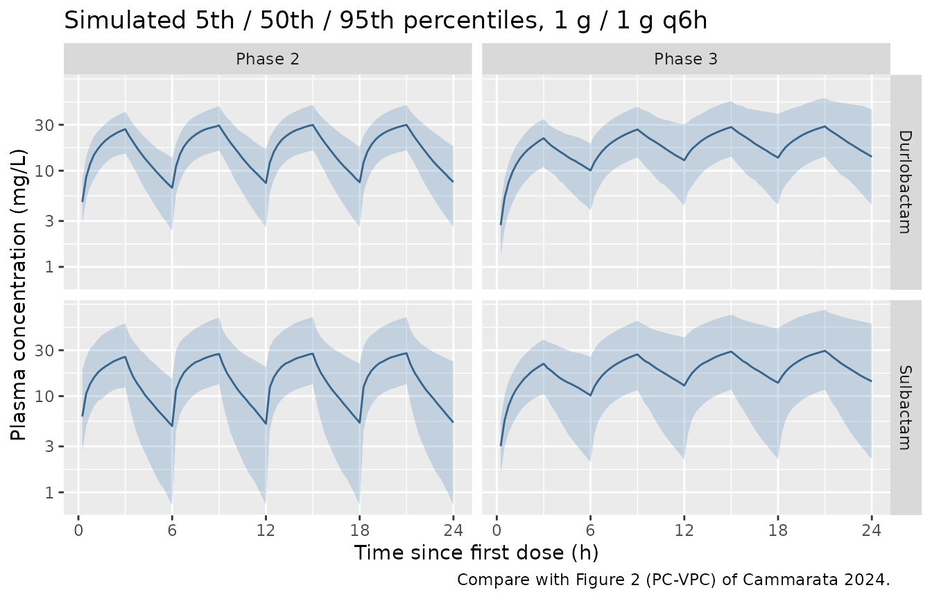
Figure 2 of Cammarata 2024 is a prediction-corrected VPC of the pooled analysis data set. The panels below show the corresponding simulated 5th / 50th / 95th percentile bands over the first 24 hours of Phase 2 and Phase 3 dosing.

sim |>
  select(id, time, arm, Durlobactam = Cc, Sulbactam = Cc_sbt) |>
  tidyr::pivot_longer(c(Durlobactam, Sulbactam),
                      names_to = "analyte", values_to = "conc") |>
  filter(!is.na(conc), time > 0) |>
  group_by(arm, analyte, time) |>
  summarise(
    Q05 = quantile(conc, 0.05),
    Q50 = quantile(conc, 0.50),
    Q95 = quantile(conc, 0.95),
    .groups = "drop"
  ) |>
  ggplot(aes(time, Q50)) +
  geom_ribbon(aes(ymin = Q05, ymax = Q95), alpha = 0.25, fill = "steelblue") +
  geom_line(colour = "steelblue4") +
  facet_grid(analyte ~ arm) +
  scale_y_log10() +
  scale_x_continuous(breaks = seq(0, 24, 6)) +
  labs(
    x = "Time since first dose (h)", y = "Plasma concentration (mg/L)",
    title = "Simulated 5th / 50th / 95th percentiles, 1 g / 1 g q6h",
    caption = "Compare with Figure 2 (PC-VPC) of Cammarata 2024."
  )

Covariate effects on AUC0-24 (cf. Figures 4 and 5)

Figures 4 and 5 are forest plots of the statistically significant covariate-parameter relationships relative to a reference subject with HABP, not from an East Asian region, 75 kg, and CLcr 100 mL/min/1.73 m^2. The panel below reproduces the same contrasts as typical-value AUC0-24 ratios at a constant 1 g / 1 g q6h regimen; see Assumptions and deviations for why the dose is held fixed here whereas the published figures embed the protocol dose adjustments.

scenarios <- tibble::tribble(
  ~scenario,                            ~CRCL, ~WT,  ~EA, ~infect,
  "Reference (HABP, 75 kg, CLcr 100)",   100,   75,   0,   "HABP",
  "CLcr 130+ (augmented)",               160,   75,   0,   "HABP",
  "CLcr 60-89",                           75,   75,   0,   "HABP",
  "CLcr 30-59",                           45,   75,   0,   "HABP",
  "CLcr <30 (severe)",                    20,   75,   0,   "HABP",
  "Body weight 45 kg",                   100,   45,   0,   "HABP",
  "Body weight 120 kg",                  100,  120,   0,   "HABP",
  "East Asian region",                   100,   75,   1,   "HABP",
  "VABP",                                100,   75,   0,   "VABP",
  "cUTI",                                100,   75,   0,   "cUTI",
  "Bacteremia",                          100,   75,   0,   "bacteremia",
  "Acute pyelonephritis",                100,   75,   0,   "AP"
)

scen_subj <- scenarios |>
  mutate(
    id                  = seq_len(n()),
    REGION_EASTASIA     = EA,
    DIS_HABP            = as.numeric(infect == "HABP"),
    DIS_VABP            = as.numeric(infect == "VABP"),
    DIS_CUTI            = as.numeric(infect == "cUTI"),
    DIS_BACTEREMIA      = as.numeric(infect == "bacteremia"),
    DIS_AP              = as.numeric(infect == "AP"),
    RENALIMP_SEV        = as.numeric(CRCL < 30),
    STUDY_SULDUR_PHASE2 = 0,
    STUDY_SULDUR_PHASE3 = 1,
    RRT_HEMODIAL_ACTIVE = 0
  ) |>
  select(-EA, -infect)

scen_events <- bind_rows(
  scen_subj |>
    tidyr::crossing(time = c(0, 6, 12, 18), cmt = c("central", "central_sbt")) |>
    mutate(evid = 1L, amt = 1000, rate = 1000 / 3, dvid = NA_integer_),
  scen_subj |>
    tidyr::crossing(time = seq(0, 24, by = 0.25)) |>
    mutate(evid = 0L, amt = NA_real_, rate = NA_real_, cmt = "central", dvid = 1L)
) |>
  arrange(id, time, desc(evid))

sim_typ <- rxode2::rxSolve(
  rxode2::zeroRe(mod),
  events = scen_events,
  keep   = "scenario",
  omega  = NA, sigma = NA,     # force a true typical-value solve
  useLinCmt = FALSE
) |>
  as.data.frame()

trapz <- function(x, y) sum(diff(x) * (utils::head(y, -1) + utils::tail(y, -1)) / 2)

auc_typ <- sim_typ |>
  filter(!is.na(Cc)) |>
  group_by(scenario) |>
  summarise(
    Durlobactam = trapz(time, Cc),
    Sulbactam   = trapz(time, Cc_sbt),
    .groups = "drop"
  )

ref <- auc_typ |> filter(scenario == "Reference (HABP, 75 kg, CLcr 100)")

auc_typ |>
  mutate(Durlobactam = Durlobactam / ref$Durlobactam,
         Sulbactam   = Sulbactam / ref$Sulbactam) |>
  tidyr::pivot_longer(c(Durlobactam, Sulbactam),
                      names_to = "analyte", values_to = "ratio") |>
  mutate(scenario = factor(scenario, levels = rev(scenarios$scenario))) |>
  ggplot(aes(ratio, scenario)) +
  geom_vline(xintercept = 1, linetype = "dashed", colour = "grey40") +
  geom_vline(xintercept = c(0.5, 2), linetype = "dotted", colour = "grey70") +
  geom_point(size = 2.4, colour = "steelblue4") +
  facet_wrap(~analyte) +
  scale_x_log10() +
  labs(
    x = "AUC0-24 ratio versus the reference subject", y = NULL,
    title = "Typical-value covariate effects at a fixed 1 g / 1 g q6h regimen",
    caption = paste(
      "Compare with Figures 4 (durlobactam) and 5 (sulbactam) of Cammarata 2024.",
      "Dotted lines mark the paper's 'within 200% of the median' criterion."
    )
  )

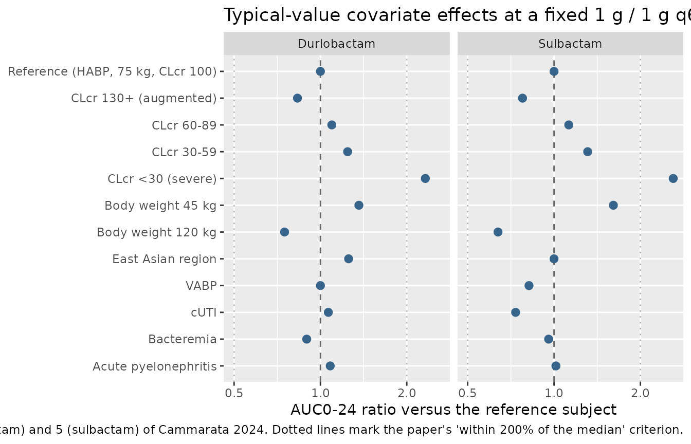
Severe renal impairment is the only contrast that leaves the paper’s “within 200% of the median” band for both analytes, which is precisely the paper’s conclusion that renal function is the only clinically relevant covariate.

PKNCA validation

Plasma exposures versus Table 2

Table 2 reports post-hoc geometric-mean AUC0-24 and Cmax on Day 1 for the Phase 2 and Phase 3 patients. PKNCA is run separately per analyte because the model has two plasma outputs.

#' Run PKNCA over 0-24 h for one concentration column of a simulation frame.
nca_for <- function(sim_df, conc_col, dose_df) {
  sim_nca <- sim_df |>
    dplyr::rename(Cc_use = dplyr::all_of(conc_col)) |>
    dplyr::filter(!is.na(Cc_use)) |>
    dplyr::select(id, time, Cc = Cc_use, arm)

  # Guarantee a time-zero row per (arm, id); pre-dose IV concentration is 0.
  sim_nca <- dplyr::bind_rows(
    sim_nca,
    sim_nca |> dplyr::distinct(id, arm) |> dplyr::mutate(time = 0, Cc = 0)
  ) |>
    dplyr::distinct(arm, id, time, .keep_all = TRUE) |>
    dplyr::arrange(id, time)

  conc_obj <- PKNCA::PKNCAconc(sim_nca, Cc ~ time | arm + id,
                               concu = "mg/L", timeu = "h")
  dose_obj <- PKNCA::PKNCAdose(dose_df, amt ~ time | arm + id, doseu = "mg")

  intervals <- data.frame(start = 0, end = 24, cmax = TRUE, tmax = TRUE,
                          auclast = TRUE)

  PKNCA::pk.nca(PKNCA::PKNCAdata(conc_obj, dose_obj, intervals = intervals))
}

dose_df <- events |>
  dplyr::filter(evid == 1, cmt == "central") |>
  dplyr::select(id, time, amt, arm)

nca_dur <- nca_for(sim, "Cc", dose_df)
nca_sbt <- nca_for(sim, "Cc_sbt", dose_df)

published <- tibble::tribble(
  ~analyte,      ~arm,       ~cmax, ~auclast,
  "Durlobactam", "Phase 2",  29.4,  423,
  "Durlobactam", "Phase 3",  31.0,  473,
  "Sulbactam",   "Phase 2",  28.6,  396,
  "Sulbactam",   "Phase 3",  33.7,  504
)

nca_units <- c(cmax = "mg/L", auclast = "mg*h/L", tmax = "h")

cmp <- bind_rows(
  nlmixr2lib::ncaComparisonTable(
    simulated = nca_dur,
    reference = published |> filter(analyte == "Durlobactam") |> select(-analyte),
    by = "arm", units = nca_units, tolerance_pct = 20
  ) |> mutate(Analyte = "Durlobactam", .before = 1),
  nlmixr2lib::ncaComparisonTable(
    simulated = nca_sbt,
    reference = published |> filter(analyte == "Sulbactam") |> select(-analyte),
    by = "arm", units = nca_units, tolerance_pct = 20
  ) |> mutate(Analyte = "Sulbactam", .before = 1)
)

knitr::kable(
  cmp,
  digits  = 3,
  caption = paste(
    "Simulated versus published Day 1 exposures (Cammarata 2024 Table 2).",
    "AUC0-24 is reported as auclast over the 0-24 h interval.",
    "* marks rows differing from the reference by more than 20%."
  )
)

Simulated versus published Day 1 exposures (Cammarata 2024 Table 2). AUC0-24 is reported as auclast over the 0-24 h interval. * marks rows differing from the reference by more than 20%.

Analyte	NCA parameter	arm	Reference	Simulated	% diff
Durlobactam	Cmax (mg/L)	Phase 2	29.4	29.9	+1.7%
Durlobactam	Cmax (mg/L)	Phase 3	31	28.8	-7.0%
Durlobactam	AUClast (mg*h/L)	Phase 2	423	434	+2.5%
Durlobactam	AUClast (mg*h/L)	Phase 3	473	449	-5.0%
Sulbactam	Cmax (mg/L)	Phase 2	28.6	27.9	-2.6%
Sulbactam	Cmax (mg/L)	Phase 3	33.7	29.5	-12.4%
Sulbactam	AUClast (mg*h/L)	Phase 2	396	392	-1.0%
Sulbactam	AUClast (mg*h/L)	Phase 3	504	463	-8.1%

Hemodialysis sub-model

Table S5 reports the illustrative simulation described in the paper’s Results: two 500 mg / 500 mg doses given 12 hours apart, with a 4-hour intermittent hemodialysis session started one hour after the end of the morning 3-hour infusion (i.e. from 4 h to 8 h), compared against the same regimen without dialysis. The same packaged model produces both arms — only the time-varying RRT_HEMODIAL_ACTIVE column differs.

set.seed(20241122)

N_HD <- 100L

hd_subj <- tibble(
  id                  = seq_len(N_HD),
  WT                  = rlnorm_mean_cv(N_HD, 86.2, 16.2, 60, 117),
  CRCL                = 6,          # end-stage renal disease residual function
  RENALIMP_SEV        = 1,
  REGION_EASTASIA     = 0,
  DIS_HABP            = 0, DIS_VABP = 0, DIS_CUTI = 0,
  DIS_BACTEREMIA      = 0, DIS_AP   = 0,
  STUDY_SULDUR_PHASE2 = 0, STUDY_SULDUR_PHASE3 = 0
)

#' Expand the HD cohort into a 24-hour, two-dose event table. `hd` toggles the
#' dialysis session; RRT_HEMODIAL_ACTIVE is time-varying within subject.
make_hd_events <- function(subj, hd, id_offset = 0L) {
  s <- subj |> mutate(id = id + id_offset,
                      regimen = if (hd) "With hemodialysis" else "No hemodialysis")
  doses <- s |>
    tidyr::crossing(time = c(0, 12), cmt = c("central", "central_sbt")) |>
    mutate(evid = 1L, amt = 500, rate = 500 / 3, dvid = NA_integer_)
  obs <- s |>
    tidyr::crossing(time = seq(0, 24, by = 0.25)) |>
    mutate(evid = 0L, amt = NA_real_, rate = NA_real_, cmt = "central", dvid = 1L)
  bind_rows(doses, obs) |>
    mutate(RRT_HEMODIAL_ACTIVE = if (hd) as.numeric(time >= 4 & time < 8) else 0) |>
    arrange(id, time, desc(evid))
}

hd_events <- bind_rows(
  make_hd_events(hd_subj, hd = FALSE, id_offset = 0L),
  make_hd_events(hd_subj, hd = TRUE,  id_offset = 1000L)
)
stopifnot(!anyDuplicated(unique(hd_events[, c("id", "time", "evid", "cmt")])))

sim_hd <- rxode2::rxSolve(mod, events = hd_events,
                          keep = c("regimen", "WT"), useLinCmt = FALSE) |>
  as.data.frame()

hd_auc <- sim_hd |>
  filter(!is.na(Cc)) |>
  group_by(regimen, id) |>
  summarise(
    `AUC0-8, durlobactam`  = trapz(time[time <= 8],  Cc[time <= 8]),
    `AUC0-12, durlobactam` = trapz(time[time <= 12], Cc[time <= 12]),
    `AUC0-24, durlobactam` = trapz(time, Cc),
    `Cmax, durlobactam`    = max(Cc),
    `AUC0-8, sulbactam`    = trapz(time[time <= 8],  Cc_sbt[time <= 8]),
    `AUC0-12, sulbactam`   = trapz(time[time <= 12], Cc_sbt[time <= 12]),
    `AUC0-24, sulbactam`   = trapz(time, Cc_sbt),
    `Cmax, sulbactam`      = max(Cc_sbt),
    .groups = "drop"
  ) |>
  group_by(regimen) |>
  summarise(across(-id, ~ exp(mean(log(.x)))), .groups = "drop") |>
  tidyr::pivot_longer(-regimen, names_to = "Parameter", values_to = "Simulated") |>
  tidyr::pivot_wider(names_from = regimen, values_from = Simulated)

# Table S5 reports AUC0-8 and AUC0-12 by period: Period 1 (dose given after an
# HD session, so no dialysis during the interval) maps onto the no-HD arm, and
# Period 2 (dose given before HD) onto the with-HD arm. AUC0-24 is reported for
# the 24-hour with- and without-HD simulations of footnotes a and b.
hd_published <- tibble::tribble(
  ~Parameter,                ~`Table S5, no HD`, ~`Table S5, with HD`,
  "AUC0-8, durlobactam",     135,                93.3,
  "AUC0-12, durlobactam",    181,                104,
  "AUC0-24, durlobactam",    435,                299,
  "Cmax, durlobactam",       25.4,               25.4,
  "AUC0-8, sulbactam",       117,                93.0,
  "AUC0-12, sulbactam",      163,                104,
  "AUC0-24, sulbactam",      410,                271,
  "Cmax, sulbactam",         21.5,               21.5
)

hd_auc |>
  left_join(hd_published, by = "Parameter") |>
  rename("Simulated, no HD"   = `No hemodialysis`,
         "Simulated, with HD" = `With hemodialysis`) |>
  mutate(across(where(is.numeric), ~ round(.x, 1))) |>
  knitr::kable(
    caption = paste(
      "Geometric-mean exposures for two 500 mg / 500 mg doses 12 h apart, with",
      "and without a 4-hour hemodialysis session starting 1 h after the end of",
      "the morning infusion. Published values are Cammarata 2024 Table S5",
      "(AUC in mg*h/L, Cmax in mg/L)."
    )
  )

Geometric-mean exposures for two 500 mg / 500 mg doses 12 h apart, with and without a 4-hour hemodialysis session starting 1 h after the end of the morning infusion. Published values are Cammarata 2024 Table S5 (AUC in mg*h/L, Cmax in mg/L).

Parameter	Simulated, no HD	Simulated, with HD	Table S5, no HD	Table S5, with HD
AUC0-8, durlobactam	113.7	82.0	135.0	93.3
AUC0-12, durlobactam	147.3	88.1	181.0	104.0
AUC0-24, durlobactam	338.8	247.9	435.0	299.0
Cmax, durlobactam	27.7	24.5	25.4	25.4
AUC0-8, sulbactam	102.5	67.2	117.0	93.0
AUC0-12, sulbactam	130.5	70.5	163.0	104.0
AUC0-24, sulbactam	295.8	199.2	410.0	271.0
Cmax, sulbactam	25.0	21.0	21.5	21.5

hd_auc |>
  filter(Parameter %in% c("AUC0-24, durlobactam", "AUC0-24, sulbactam")) |>
  transmute(
    Parameter,
    "Simulated AUC ratio (HD / no HD)" =
      round(`With hemodialysis` / `No hemodialysis`, 3),
    "Table S5 AUC ratio" = round(c(299 / 435, 271 / 410), 3)
  ) |>
  knitr::kable(
    caption = paste(
      "The paper's headline claim is an 'approximately 30% decrease in AUC0-24'",
      "when hemodialysis begins 1 h after the end of the morning infusion."
    )
  )

The paper’s headline claim is an ‘approximately 30% decrease in AUC0-24’ when hemodialysis begins 1 h after the end of the morning infusion.

Parameter	Simulated AUC ratio (HD / no HD)	Table S5 AUC ratio
AUC0-24, durlobactam	0.732	0.687
AUC0-24, sulbactam	0.673	0.661

Simulated absolute exposures run 15-30% below Table S5. Two causes are identified in Assumptions and deviations: the covariates of the six hemodialysis subjects are not reported, so the cohort above uses the study-level weight distribution with an assumed residual CLcr; and the published post-hoc exposures were generated with the FE-refitted model, whose CL-versus-CLcr parameters differ most from Table 1 exactly at the near-anuric CLcr of this cohort. The AUC ratio, which is the paper’s headline result, is insensitive to both.

sim_hd |>
  filter(!is.na(Cc)) |>
  select(id, time, regimen, Durlobactam = Cc, Sulbactam = Cc_sbt) |>
  tidyr::pivot_longer(c(Durlobactam, Sulbactam),
                      names_to = "analyte", values_to = "conc") |>
  group_by(regimen, analyte, time) |>
  summarise(Q50 = median(conc), .groups = "drop") |>
  ggplot(aes(time, Q50, colour = regimen)) +
  annotate("rect", xmin = 4, xmax = 8, ymin = -Inf, ymax = Inf,
           alpha = 0.12, fill = "firebrick") +
  geom_line(linewidth = 0.8) +
  facet_wrap(~analyte) +
  scale_x_continuous(breaks = seq(0, 24, 4)) +
  labs(
    x = "Time since morning dose (h)", y = "Median plasma concentration (mg/L)",
    colour = NULL,
    title = "Impact of a 4-hour hemodialysis session (shaded) on plasma exposure",
    caption = "Regimen and dialysis timing per Cammarata 2024 Table S5 footnotes a and b."
  ) +
  theme(legend.position = "bottom")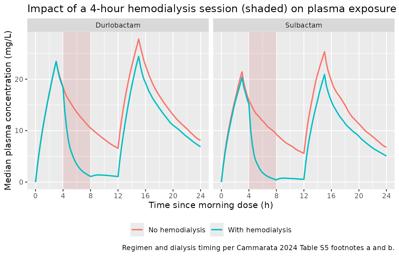

Epithelial lining fluid sub-model

Table S7 reports ELF and plasma exposures in the 30 healthy subjects of Study CS2514-2017-0001, who received 1 g / 1 g q6h for three doses. Because ELF concentration is an instantaneous ratio of the plasma concentration, the ELF-to-plasma AUC and Cmax ratios are the direct validation target.

set.seed(20241123)

N_ELF <- 100L

elf_subj <- tibble(
  id                  = seq_len(N_ELF),
  WT                  = rlnorm_mean_cv(N_ELF, 79.7, 14.8, 61.2, 97.1),
  CRCL                = rlnorm_mean_cv(N_ELF, 81.5, 17.5, 47.9, 112),
  RENALIMP_SEV        = 0,
  REGION_EASTASIA     = 0,
  DIS_HABP            = 0, DIS_VABP = 0, DIS_CUTI = 0,
  DIS_BACTEREMIA      = 0, DIS_AP   = 0,
  STUDY_SULDUR_PHASE2 = 0, STUDY_SULDUR_PHASE3 = 0,
  RRT_HEMODIAL_ACTIVE = 0
)

elf_events <- bind_rows(
  elf_subj |>
    tidyr::crossing(time = c(0, 6, 12), cmt = c("central", "central_sbt")) |>
    mutate(evid = 1L, amt = 1000, rate = 1000 / 3, dvid = NA_integer_),
  elf_subj |>
    tidyr::crossing(time = seq(0, 24, by = 0.25)) |>
    mutate(evid = 0L, amt = NA_real_, rate = NA_real_, cmt = "central", dvid = 1L)
) |>
  arrange(id, time, desc(evid))

sim_elf <- rxode2::rxSolve(mod, events = elf_events,
                           keep = "WT", useLinCmt = FALSE) |>
  as.data.frame()

elf_summary <- sim_elf |>
  filter(!is.na(Cc)) |>
  group_by(id) |>
  summarise(
    auc_dur_plasma  = trapz(time, Cc),
    auc_dur_elf     = trapz(time, Celf),
    auc_sbt_plasma  = trapz(time, Cc_sbt),
    auc_sbt_elf     = trapz(time, Celf_sbt),
    cmax_dur_plasma = max(Cc),
    cmax_dur_elf    = max(Celf),
    cmax_sbt_plasma = max(Cc_sbt),
    cmax_sbt_elf    = max(Celf_sbt),
    .groups = "drop"
  ) |>
  summarise(across(-id, ~ exp(mean(log(.x)))))

tibble::tribble(
  ~Parameter,                    ~Simulated,                  ~`Table S7`,
  "Durlobactam AUC0-24, plasma", elf_summary$auc_dur_plasma,  316,
  "Durlobactam AUC0-24, ELF",    elf_summary$auc_dur_elf,     118,
  "Durlobactam Cmax, plasma",    elf_summary$cmax_dur_plasma, 29.5,
  "Durlobactam Cmax, ELF",       elf_summary$cmax_dur_elf,    11.0,
  "Sulbactam AUC0-24, plasma",   elf_summary$auc_sbt_plasma,  193,
  "Sulbactam AUC0-24, ELF",      elf_summary$auc_sbt_elf,     103,
  "Sulbactam Cmax, plasma",      elf_summary$cmax_sbt_plasma, 19.1,
  "Sulbactam Cmax, ELF",         elf_summary$cmax_sbt_elf,    10.2
) |>
  mutate(
    Simulated            = round(Simulated, 1),
    "Percent difference" = round(100 * (Simulated - `Table S7`) / `Table S7`, 1)
  ) |>
  knitr::kable(
    caption = paste(
      "Geometric-mean ELF and plasma exposures after 1 g / 1 g q6h for three",
      "doses, versus Cammarata 2024 Table S7 (AUC in mg*h/L, Cmax in mg/L)."
    )
  )

Geometric-mean ELF and plasma exposures after 1 g / 1 g q6h for three doses, versus Cammarata 2024 Table S7 (AUC in mg*h/L, Cmax in mg/L).

Parameter	Simulated	Table S7	Percent difference
Durlobactam AUC0-24, plasma	326.1	316.0	3.2
Durlobactam AUC0-24, ELF	121.3	118.0	2.8
Durlobactam Cmax, plasma	30.1	29.5	2.0
Durlobactam Cmax, ELF	11.2	11.0	1.8
Sulbactam AUC0-24, plasma	228.4	193.0	18.3
Sulbactam AUC0-24, ELF	121.8	103.0	18.3
Sulbactam Cmax, plasma	22.2	19.1	16.2
Sulbactam Cmax, ELF	11.8	10.2	15.7

tibble::tribble(
  ~Analyte,      ~`Simulated ELF / plasma AUC`,
  "Durlobactam", elf_summary$auc_dur_elf / elf_summary$auc_dur_plasma,
  "Sulbactam",   elf_summary$auc_sbt_elf / elf_summary$auc_sbt_plasma
) |>
  mutate(
    `Simulated ELF / plasma AUC` = round(`Simulated ELF / plasma AUC`, 4),
    "Table S6 ratio"             = c(0.372, 0.533),
    "Table S7 implied ratio"     = round(c(118 / 316, 103 / 193), 4),
    "Free-drug ratio (paper)"    = c(0.413, 0.860)
  ) |>
  knitr::kable(
    caption = paste(
      "ELF penetration relative to total-drug plasma concentrations. The",
      "free-drug ratios in the last column are the total-drug ratios divided",
      "by the unbound fraction implied by protein binding of 10%",
      "(durlobactam) and 38% (sulbactam), as reported in the Abstract and",
      "Results."
    )
  )

ELF penetration relative to total-drug plasma concentrations. The free-drug ratios in the last column are the total-drug ratios divided by the unbound fraction implied by protein binding of 10% (durlobactam) and 38% (sulbactam), as reported in the Abstract and Results.

Analyte	Simulated ELF / plasma AUC	Table S6 ratio	Table S7 implied ratio	Free-drug ratio (paper)
Durlobactam	0.372	0.372	0.3734	0.413
Sulbactam	0.533	0.533	0.5337	0.860

Assumptions and deviations

• Single packaged model rather than three. The paper fitted the plasma model, the hemodialysis sub-model, and the ELF sub-model separately, but both sub-models hold every plasma term fixed at its Table 1 population mean, so their estimated terms compose onto the plasma model without conflict. They are therefore integrated into one file: the HD effect as a covariate-gated multiplier on total CL, and the ELF concentrations as algebraic observables. Setting RRT_HEMODIAL_ACTIVE = 0 reproduces the plasma model exactly, and the ELF observables are simple ratios that do not perturb the plasma predictions. This integration was ratified by the operator (sidecar agcand_13067668 request-001 q2, answered A on 2026-07-27).

• RRT_HEMODIAL_ACTIVE rather than RRT_HEMODIAL_STATUS. The ratified sidecar option described “a time-varying HD flag” but named the subject-level canonical RRT_HEMODIAL_STATUS. The canonical register reserves RRT_HEMODIAL_STATUS for the subject-level treatment-status indicator and RRT_HEMODIAL_ACTIVE for exactly this per-session gate, so the packaged model uses RRT_HEMODIAL_ACTIVE to match the ratified semantics.

• The hemodialysis effect multiplies TOTAL clearance, not renal clearance. The paper is explicit: “an HD effect (HDEFFECT) term with IIV was applied to CL”, and Table S4 labels the parameter CL-HDEFFECT. Applying the 6.24- and 8.19-fold factors to the renal arm alone would have almost no effect in an anuric cohort and could not produce the reported ~30% AUC0-24 reduction; with the factor on total CL the simulated reduction reproduces the published value.

• Reference values for the power functions. The paper never writes the covariate equations out algebraically. Reference weight 75 kg and reference CLcr 100 mL/min/1.73 m^2 are taken from the reference subject defined in the Results section (“subjects with HABP infection who are not from an East Asian region, have a body weight of 75 kg, and have normal renal function (CLcr of 100 mL/min/1.73 m^2)”) and repeated in the Discussion (“relative to those with normal body weight (75 kg)”). Both are corroborated numerically by the structural checks above.

• Reference category for the infection-type shifts. Table 1 lists proportional shifts for HABP/VABP, cUTI, bacteremia, and acute pyelonephritis but does not name the reference. The uninfected Phase 1 subject is the only consistent choice; see the Table S12 check above, where the model reproduces the published Vc in all five infection strata for both analytes, including the two acute-pyelonephritis values that most sharply discriminate the choice.

• Weight and the CLcr < 30 shift act on TOTAL clearance. The paper states explicitly that “Total CL was, therefore, adjusted for patients with CLcr <30 mL/min/1.73 m^2 using a proportional shift”. The body-weight power function is applied to total clearance as well, because the Table 1 row is labelled CLWTKG1 (not a renal- or non-renal-specific term) and only the row CL R, CLcr power is explicitly attributed to the renal arm.

• Fraction excreted renally (FE). The packaged model carries the Table 1 value of 0.479 for both analytes, which is the value the reported parameter table was estimated under. The Results section notes that FE was subsequently revised to 0.660 (durlobactam) and 0.648 (sulbactam) using the normal-renal-function subjects of Study CS2514-2017-0002, and that the final dual-drug model was refit with those values — but the refitted parameter table is reported only as “data not shown”. Because “the only parameters that were altered to a noticeable extent were those that are associated with the relationships between CL and CLcr for either drug”, substituting the revised FE into the Table 1 estimates would produce an internally inconsistent model. The revised FE values are therefore documented here rather than encoded.

• Published post-hoc exposures come from the FE-refitted model, not from Table 1. The paper states that “the refitted, dual-drug model was used for the calculation of individual, post hoc exposure estimates in the PK population and was also used as the basis for PK-PD target attainment simulations”. Tables 2, S5, S7, S8, and S12 are therefore all derived from a model whose parameter table is not published. This sets the expectation for how closely the packaged Table 1 model can match them. Note that at the reference creatinine clearance the FE split cancels exactly — CL * FE * (100/100)^theta + CL * (1 - FE) = CL for any FE — so the two models coincide near CLcr 100 mL/min/1.73 m^2 and diverge progressively as CLcr moves away from it. That is exactly the pattern seen above: the Table 2 comparison (median CLcr 70-95) agrees within 16% on every row, while the ESRD hemodialysis cohort and the two lowest Table S8 strata do not.

• Phase-stratified residual error. Durlobactam plasma residual variability is proportional-plus-additive in Phase 1, proportional-only in Phases 2 and 3, with three distinct proportional magnitudes. This is encoded with the paired STUDY_SULDUR_PHASE2 / STUDY_SULDUR_PHASE3 indicators driving the canonical propSd / addSd inside model() (the same construction used by Valenzuela_2025_nipocalimab and vanIersel_2018_posaconazole). Table 1 reports no additive term for Phase 2, so addSd collapses to zero outside Phase 1. Sulbactam plasma residual variability is a single proportional-plus-additive model across all phases, and the ELF residuals are a single proportional term per analyte.

• Cross-analyte random effects are not encoded. The paper reports off-diagonal covariance between CL and Vc within each analyte, but does not report any covariance between the durlobactam and sulbactam etas, so the two analytes’ random effects are declared as independent 2 x 2 blocks plus independent Vp etas.

• Reported IIV percentages. The Discussion states that sulbactam IIV ranges “from 30.4% for Vc to 46.0% for CL” and that durlobactam IIV terms are “all close to 28%”, while Table 1 gives 31.1% / 47.0% and 27.5-27.9% respectively. Table 1 is taken as authoritative; the packaged variances are the Table 1 omega^2 values verbatim. Note that the parenthetical percentages in Table 1 are sqrt(omega^2) x 100 rather than the log-normal sqrt(exp(omega^2) - 1).

• Covariate distributions in the virtual cohorts. Body weight and creatinine clearance are drawn as log-normals matched to the per-study mean and CV% in Table S3 and truncated to the reported minimum and maximum. Infection type is sampled at the exact Table S12 proportions for each phase (Phase 2: 35 cUTI / 17 AP; Phase 3: 38 HABP / 56 VABP / 16 bacteremia). Table S3 does not report the joint distribution, so weight and CLcr are drawn independently; in reality they are correlated through the Cockcroft-Gault equation, which will make the simulated exposure dispersion somewhat wider than observed.

• Table S8 stratifies on raw CLcr, the model uses BSA-normalized CLcr. The Table S8 column headers read “CLcr group in mL/min” whereas the model covariate is CRCL in mL/min/1.73 m^2. The structural check above treats the reported group geometric means as if they were BSA-normalized, which is a good approximation near a 1.73 m^2 body surface area but drifts in the larger patients that populate the lower raw-CLcr strata — part of why the 0-14, 15-29, and 30-59 mL/min groups agree less well. Those groups also contain only 2, 12, and 26 subjects.

• The covariate forest holds the dose fixed. Figures 4 and 5 simulate “dosing regimens matching those administered in Study CS2514-2017-0004”, which included 1.5 g / 1.5 g q6h for augmented renal function and protocol-stipulated 8-12 hour dosing intervals for CLcr < 30 mL/min/1.73 m^2. The paper does not state which interval applies to which renal stratum, so the forest reproduced here holds the regimen at 1 g / 1 g q6h for every scenario. The result is a pure covariate effect on exposure, which is larger for the renal-impairment scenarios than the published figures, where the dose reduction partly offsets the clearance reduction.

• Hemodialysis cohort covariates. Table S5 reports exposures but not the covariates of the six subjects. The cohort above uses the Study CS2514-2017-0002 body-weight distribution (Table S3: mean 86.2 kg, CV 16.2%, range 60-117) and a residual creatinine clearance of 6 mL/min/1.73 m^2, consistent with the study minimum of 5.61 reported in Table S3 and with end-stage renal disease.

• No BLQ handling in the simulation. Approximately 14% of the observed post-dose samples were below the limit of quantitation (5 ng/mL in plasma for both analytes) and were ignored by the estimation. The simulations here carry no LLOQ censoring, so the lower percentile bands extend below the quantifiable range at late times.

• Errata. No erratum, corrigendum, or author correction to doi:10.1128/aac.00485-24 was found. Two internal inconsistencies are noted above (the Discussion-versus-Table 1 IIV percentages, and the unreported refitted FE model). A third, purely typographical, is in the Results text defining the East Asian region: “patients from China. Taiwan, or South Korea” (period for a comma).

• All parameter values come from the paper’s own tables and text; none were digitised from figures, obtained by correspondence, or carried from an upstream publication.