Enrofloxacin and ciprofloxacin in cats (Foster 2023)
Source:vignettes/articles/Foster_2023_enrofloxacin_cat.Rmd
Foster_2023_enrofloxacin_cat.RmdModels and source
- Citation: Foster JD, Abouraya M, Papich MG, Muma NA. (2023). Population pharmacokinetic analysis of enrofloxacin and its active metabolite ciprofloxacin after intravenous injection to cats with reduced kidney function. Journal of Veterinary Internal Medicine 37(6):2230-2240. doi:10.1111/jvim.16866.
- Article: J Vet Intern Med 37(6):2230-2240
Foster and colleagues gave a single 5 mg/kg intravenous dose of enrofloxacin, infused over 30 minutes, to 34 client-owned cats hospitalised for clinical illness and spanning the full range from normal kidney function to severe azotemia, then used sparse sampling (three plasma samples per cat) and nonlinear mixed-effects modelling in Phoenix NLME to answer a single clinical question: does enrofloxacin accumulate in azotemic cats? It does not, and the paper’s conclusion is that no dosage adjustment is indicated.
The paper reports two independent fits of the same study data, and this package carries them as two model files pointing at this one vignette.
| Model file | Fitted to | Structure | Retained covariates |
|---|---|---|---|
Foster_2023_enrofloxacin_totalFluoroquinolone_cat |
the sum of plasma enrofloxacin and ciprofloxacin (“total fluoroquinolone”) | 2-compartment | body weight on V1 and Cl1 |
Foster_2023_enrofloxacin_ciprofloxacin_cat |
enrofloxacin and ciprofloxacin measured separately | 1 compartment per analyte, coupled by a metabolic formation clearance | body weight on the enrofloxacin volume; BUN on the formation clearance |
The two are not nested: the first is the paper’s primary analysis (Results 3.1 to 3.3, Table 1) and the second is a secondary analysis of ciprofloxacin generation (Results 3.4, Figure S2, Tables 2 and 3). They are extracted as separate files because the authors fitted them separately.
Ciprofloxacin is the principal active metabolite of enrofloxacin, formed by hepatic N-dealkylation, and the two compounds’ antibacterial effects are additive – which is why the authors’ primary analyte is their sum.
Population
Thirty-four client-owned cats (18 spayed females, 16 castrated males), mean age 11.4 +/- 4.3 years, median body weight 3.8 kg (range 1.8-8.8 kg), enrolled at a single referral hospital between 1 January 2019 and 1 September 2021. Nine cats had normal kidney function (median serum creatinine 1.6 mg/dL, range 0.9-2.2), 15 had moderate kidney dysfunction (median 5.6, range 2.7-8.6) and 10 had severe kidney dysfunction (median 13.3, range 11.9-21.5). Cohort mean serum creatinine was 7.5 +/- 6.0 mg/dL, BUN 137.6 +/- 103.0 mg/dL and SDMA 39.8 +/- 27.0 ug/dL.
Every cat received 5 mg/kg enrofloxacin (Baytril 2.27%, Elanco) diluted 1:1 with sterile saline and infused intravenously over 30 minutes through a peripheral catheter; the mean total dose was 20.5 +/- 7.4 mg. Each cat was scheduled for three plasma samples in the 24 hours after dosing, randomly assigned to one of seven optimised sparse-sampling schedules; 98 samples were analysed (four cats contributed only two usable samples). Enrofloxacin and ciprofloxacin were quantified separately by validated HPLC, which is what makes the parent + metabolite fit possible.
The same information is available programmatically from either
model’s population metadata, e.g.
readModelDb("Foster_2023_enrofloxacin_totalFluoroquinolone_cat")()$population.
Units: the parameters are absolute, not per kilogram
Foster 2023 labels every volume in Tables 1, 2 and 3 as “mL/kg” and every clearance as “mL/kg/h”. Those parameters are absolute (mL and mL/h), and both model files encode them that way, with doses entered as the total amount in ug. This is the single most consequential decision in the extraction, so the arithmetic is set out here rather than buried in the Errata.
Reading Table 1 as absolute and using the cohort’s mean total dose of 20.5 mg = 20500 ug:
v1 <- 4794.7   # Table 1 theta Vd1
cl1 <- 254.3   # Table 1 theta Cl1
q <- 132.1     # Table 1 Cl2
v2 <- 2.9e4    # Table 1 Vd2

# Analytic 2-compartment AUC after a bolus, absolute reading, 20500 ug.
k10 <- cl1 / v1; k12 <- q / v1; k21 <- q / v2
sum_rate <- k10 + k12 + k21
disc <- sqrt(sum_rate^2 - 4 * k10 * k21)
alpha <- (sum_rate + disc) / 2
beta <- (sum_rate - disc) / 2
c0 <- 20500 / v1
a <- c0 * (alpha - k21) / (alpha - beta)
b <- c0 - a

tibble::tibble(
  Quantity = c(
    "C(0) (ug/mL)", "AUC0-inf (h*ug/mL)", "AUC0-24 (h*ug/mL)",
    "Dose / AUC0-24 (mL/h)"
  ),
  `Absolute reading (mL, mL/h)` = c(
    c0,
    a / alpha + b / beta,
    a / alpha * (1 - exp(-24 * alpha)) + b / beta * (1 - exp(-24 * beta)),
    20500 / (a / alpha * (1 - exp(-24 * alpha)) + b / beta * (1 - exp(-24 * beta)))
  ),
  `Per-kilogram reading` = c(
    5000 / v1,
    (a / alpha + b / beta) * 5000 / 20500,
    (a / alpha * (1 - exp(-24 * alpha)) + b / beta * (1 - exp(-24 * beta))) *
      5000 / 20500,
    NA_real_
  ),
  `Published` = c(NA_real_, NA_real_, 46.0, 440.8)
) |>
knitr::kable(digits = 2)| Quantity | Absolute reading (mL, mL/h) | Per-kilogram reading | Published |
|---|---|---|---|
| C(0) (ug/mL) | 4.28 | 1.04 | NA |
| AUC0-inf (h*ug/mL) | 80.61 | 19.66 | NA |
| AUC0-24 (h*ug/mL) | 45.89 | 11.19 | 46.0 |
| Dose / AUC0-24 (mL/h) | 446.76 | NA | 440.8 |
The absolute reading reproduces Table 1’s AUC0-24 of 46.0 h*ug/mL to within 0.3%, reproduces the “observed clearance” median of 440.8 reported in Results 3.1, and puts the initial concentration at about 4.3 ug/mL, inside the 3-8 ug/mL band in which Figure 1’s spaghetti plot starts. The per-kilogram reading is four-fold low on every one of those quantities. The same check on the parent + metabolite model gives an enrofloxacin C(0) of 20500 / 5797.5 = 3.5 ug/mL under the absolute reading versus 0.86 ug/mL under the per-kilogram reading.
The absolute reading also makes the fitted weight exponents interpretable: an exponent near 1 on an absolute volume is ordinary body-size scaling, whereas the same exponent stacked on an already-per-kilogram volume would mean total scaling with WT to the power 2.63.
Source trace
The per-parameter origin is recorded as an in-file comment next to
each ini() entry in both model files. The table below
collects them in one place.
Foster_2023_enrofloxacin_totalFluoroquinolone_cat
| Equation / parameter | Value as published | Value in ini()
|
Source location |
|---|---|---|---|
lvc |
theta Vd1 = 4794.7 (SE 359.6, CV% 7.22) |
log(4794.7) mL |
Table 1 |
lvp |
Vd2 = 2.9 x 10^4 (SE 5.1 x 10^5) |
log(2.9e4) mL |
Table 1 |
lcl |
theta Cl1 = 254.3 (SE 31.8, CV% 12.49) |
log(254.3) mL/h |
Table 1 |
lq |
Cl2 = 132.1 (SE 27.4, CV% 20.71) |
log(132.1) mL/h |
Table 1 |
e_wt_vc |
effect 1.63, SE 0.19 (Table 1 prints 1.6) | 1.63 |
Abstract, Results; Table 1 dVd1weight
|
e_wt_cl |
effect 1.63, SE 0.27 (Table 1 prints 1.6) | 1.63 |
Abstract, Results; Table 1 dCl1weight
|
| weight centring | “body weight was centered around the mean population body weight, 3.8 kg” | (WT / 3.8)^e |
Results 3.2 |
all eta*
|
exponential IIV stated; no variances published | fixed(0) |
Methods para. 7; Figures 2 and 3 plot the etas |
propSd |
multiplicative residual model selected on AIC; no sigma published | fixed(0) |
Methods para. 7; Results 3.1 |
d/dt(central), d/dt(peripheral1)
|
2-compartment, Cl1 out of compartment 1, Cl2 between compartments | n/a | Results 3.1, Table 1 note |
Foster_2023_enrofloxacin_ciprofloxacin_cat
| Equation / parameter | Value as published | Value in ini()
|
Source location |
|---|---|---|---|
lvc |
theta Vd enrofloxacin = 5797.5 (SE 313.5, CV% 5.4) |
log(5797.5) mL |
Table 3 (Table 2 identical) |
lcl_nonmet |
clearance of enrofloxacin into urine = 499.1 (SE 42.6, CV% 8.5) |
log(499.1) mL/h |
Table 3 (Table 2 identical) |
lcl_met |
metabolism of enrofloxacin to ciprofloxacin = 0.13 (SE 0.03, CV% 22.9) |
log(0.13) mL/h |
Table 2; Table 3 prints the same parameter rounded to 0.1 |
lvc_cipro |
Vd ciprofloxacin = 22.6 (SE 4.2, CV% 18.7) |
log(22.6) mL |
Table 3 (Table 2 gives 22.7) |
lcl_cipro |
clearance of ciprofloxacin into urine = 4.6 (SE 0.8, CV% 16.9) |
log(4.6) mL/h |
Table 3 (Table 2 identical) |
e_wt_vc |
dVd Enrofloxacin-Weight = 0.7 (SE 0.15, CV% 20.0) | 0.7 |
Table 3 |
e_bun_cl_met |
effect 0.51, SE 0.08 (Table 3 prints 0.5) | 0.51 |
Abstract; Table 3 dCl ... BUN
|
| BUN centring | not stated by the paper; cohort mean used | (BUN / 137.6)^e |
Results section 3 (cohort mean BUN); see Errata |
all eta*
|
exponential IIV stated; no variances published | fixed(0) |
Methods para. 7; Figure 5 plots all five etas |
propSd, propSd_cipro
|
multiplicative residual model; no sigma published | fixed(0) |
Methods para. 7 |
d/dt(central), d/dt(central_cipro)
|
enrofloxacin cleared to urine and metabolised to ciprofloxacin; ciprofloxacin cleared to urine | n/a | Figure S2 (graphical model), Results 3.4 |
Ciprofloxacin enters the register of metabolite / sibling-drug
suffixes as cipro
(inst/references/compartment-names.md), giving the
compartment central_cipro, the parameters
lvc_cipro / lcl_cipro and the output
Cc_cipro.
Virtual cohort
The original per-cat data are not publicly available. The cohort below reconstructs the 34 cats from the published marginal summaries: body weights are the quantiles of a log-normal with median 3.8 kg chosen so the extremes land near the reported 1.8-8.8 kg range, and BUN values are the quantiles of a log-normal matching the reported mean of 137.6 mg/dL and SD of 103.0 mg/dL. Because no between-subject variances were published (see Errata), these covariates are the only source of between-cat spread in the simulations.
n_cats <- 34L

cohort <- tibble(
  id = seq_len(n_cats),
  WT = round(qlnorm(ppoints(n_cats), meanlog = log(3.8), sdlog = 0.38), 2),
  BUN = round(qlnorm(ppoints(n_cats), meanlog = log(137.6) - 0.6673^2 / 2,
                     sdlog = 0.6673), 1)
) |>
  mutate(dose_ug = 5 * WT * 1000)

tibble(
  Quantity = c("Body weight (kg)", "BUN (mg/dL)", "Total dose (mg)"),
  Published = c("median 3.8, range 1.8-8.8", "mean 137.6 +/- 103.0",
                "mean 20.5 +/- 7.4"),
  Simulated = c(
    sprintf("median %.1f, range %.1f-%.1f", median(cohort$WT),
            min(cohort$WT), max(cohort$WT)),
    sprintf("mean %.1f +/- %.1f", mean(cohort$BUN), sd(cohort$BUN)),
    sprintf("mean %.1f +/- %.1f", mean(cohort$dose_ug) / 1000,
            sd(cohort$dose_ug) / 1000)
  )
) |>
knitr::kable()| Quantity | Published | Simulated |
|---|---|---|
| Body weight (kg) | median 3.8, range 1.8-8.8 | median 3.8, range 1.7-8.7 |
| BUN (mg/dL) | mean 137.6 +/- 103.0 | mean 136.1 +/- 95.8 |
| Total dose (mg) | mean 20.5 +/- 7.4 | mean 20.4 +/- 7.9 |
Simulation
All simulations use rxode2::zeroRe(). Every eta and both
residual SDs are fixed(0) because Foster 2023 publishes no
variance components (see Errata), so the models produce deterministic
typical-value profiles; zeroRe() makes that explicit and
keeps rxSolve() from attempting a Cholesky factorisation of
a zero omega matrix.
mod_tfq <- rxode2::zeroRe(
  readModelDb("Foster_2023_enrofloxacin_totalFluoroquinolone_cat")
)
mod_met <- rxode2::zeroRe(
  readModelDb("Foster_2023_enrofloxacin_ciprofloxacin_cat")
)

inf_dur <- 0.5  # 30-minute infusion, Methods para. 3
obs_times <- sort(unique(c(seq(0, 24, by = 0.02), inf_dur)))

events_tfq <- bind_rows(
  cohort |>
    transmute(id, WT, time = 0, amt = dose_ug, rate = dose_ug / inf_dur,
              evid = 1L, cmt = "central"),
  cohort |>
    select(id, WT) |>
    crossing(time = obs_times) |>
    mutate(amt = NA_real_, rate = NA_real_, evid = 0L, cmt = "central")
) |>
  arrange(id, time, desc(evid))

sim_tfq <- rxode2::rxSolve(
  mod_tfq, events = events_tfq, returnType = "data.frame"
) |>
  filter(!is.na(Cc))
#> ℹ omega/sigma items treated as zero: 'etalvc', 'etalvp', 'etalcl', 'etalq'
#> Warning: multi-subject simulation without without 'omega'

# rxSolve silently drops subjects when an event table is malformed; assert.
stopifnot(length(unique(sim_tfq$id)) == n_cats)
Replicates Figure 1 of Foster 2023
Figure 1 of the paper is a semilogarithmic spaghetti plot of the observed total fluoroquinolone concentrations in all 34 cats over 24 hours, on a 0.1-10 ug/mL axis. The simulated profiles below are plotted on the same axes. The observed plot has more spread, because the published spread contains between-subject and residual variability that the packaged model cannot reproduce; the simulated fan comes from body weight alone.
ggplot(sim_tfq |> filter(time > 0), aes(time, Cc, group = id)) +
  geom_line(linewidth = 0.4, alpha = 0.7) +
  scale_y_log10(
    limits = c(0.1, 10), breaks = c(0.1, 1, 10),
    labels = c("0.1", "1", "10")
  ) +
  scale_x_continuous(limits = c(0, 25), breaks = seq(0, 25, by = 5)) +
  labs(
    x = "Time (hours)",
    y = "Total fluoroquinolone plasma concentration (ug/mL)"
  ) +
  theme_bw()
#> Warning: Removed 1 row containing missing values or values outside the scale range
#> (`geom_line()`).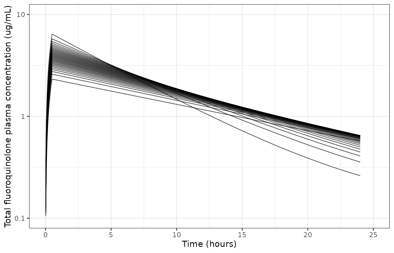
Replicates Figure 1 of Foster 2023: total fluoroquinolone plasma concentration over 24 h after a single 5 mg/kg intravenous enrofloxacin dose in 34 cats.
tibble(
  Quantity = c(
    "Concentration just after the infusion (ug/mL)",
    "Concentration at 24 h (ug/mL)"
  ),
  `Figure 1 (observed, read off the axes)` = c("about 3 to 8", "about 0.2 to 3"),
  Simulated = c(
    sprintf("%.2f to %.2f",
            min(sim_tfq$Cc[abs(sim_tfq$time - inf_dur) < 1e-8]),
            max(sim_tfq$Cc[abs(sim_tfq$time - inf_dur) < 1e-8])),
    sprintf("%.2f to %.2f",
            min(sim_tfq$Cc[sim_tfq$time == 24]),
            max(sim_tfq$Cc[sim_tfq$time == 24]))
  )
) |>
knitr::kable()| Quantity | Figure 1 (observed, read off the axes) | Simulated |
|---|---|---|
| Concentration just after the infusion (ug/mL) | about 3 to 8 | 2.32 to 6.42 |
| Concentration at 24 h (ug/mL) | about 0.2 to 3 | 0.26 to 0.65 |
PKNCA validation
Non-compartmental analysis of the simulated profiles, computed with
PKNCA over the 0-24 h window the paper used. Three arms are
analysed together: the total fluoroquinolone model for the typical 3.8
kg cat, and the two analytes of the parent + metabolite model for the
same cat at the cohort mean BUN.
typ_wt <- 3.8
typ_bun <- 137.6
typ_dose <- 5 * typ_wt * 1000

ev_typ_tfq <- bind_rows(
  tibble(id = 1L, WT = typ_wt, time = 0, amt = typ_dose,
         rate = typ_dose / inf_dur, evid = 1L, cmt = "central"),
  tibble(id = 1L, WT = typ_wt, time = obs_times, amt = NA_real_,
         rate = NA_real_, evid = 0L, cmt = "central")
) |>
  arrange(time, desc(evid))

# The parent + metabolite model declares two endpoints (Cc and Cc_cipro), so
# observation records must name an endpoint; rxode2 returns both output
# columns on every observation row.
ev_typ_met <- bind_rows(
  tibble(id = 1L, WT = typ_wt, BUN = typ_bun, time = 0, amt = typ_dose,
         rate = typ_dose / inf_dur, evid = 1L, cmt = "central"),
  tibble(id = 1L, WT = typ_wt, BUN = typ_bun, time = obs_times,
         amt = NA_real_, rate = NA_real_, evid = 0L, cmt = "Cc")
) |>
  arrange(time, desc(evid))

sim_typ_tfq <- rxode2::rxSolve(
  mod_tfq, events = ev_typ_tfq, returnType = "data.frame"
) |>
  filter(!is.na(Cc))
#> ℹ omega/sigma items treated as zero: 'etalvc', 'etalvp', 'etalcl', 'etalq'
sim_typ_met <- rxode2::rxSolve(
  mod_met, events = ev_typ_met, returnType = "data.frame"
) |>
  filter(!is.na(Cc))
#> ℹ omega/sigma items treated as zero: 'etalvc', 'etalcl_nonmet', 'etalcl_met', 'etalvc_cipro', 'etalcl_cipro'

conc_all <- bind_rows(
  sim_typ_tfq |>
    transmute(id = 1L, time, conc = Cc, arm = "Total fluoroquinolone"),
  sim_typ_met |>
    transmute(id = 1L, time, conc = Cc, arm = "Enrofloxacin"),
  sim_typ_met |>
    transmute(id = 1L, time, conc = Cc_cipro, arm = "Ciprofloxacin")
)

dose_all <- tibble(
  id = 1L, time = 0, amt = typ_dose,
  arm = c("Total fluoroquinolone", "Enrofloxacin", "Ciprofloxacin")
)

nca_all <- as.data.frame(
  PKNCA::pk.nca(
    PKNCA::PKNCAdata(
      PKNCA::PKNCAconc(conc_all, conc ~ time | arm + id,
                       concu = "ug/mL", timeu = "h"),
      PKNCA::PKNCAdose(dose_all, amt ~ time | arm + id,
                       doseu = "ug", route = "intravascular"),
      intervals = data.frame(
        start = 0, end = 24,
        cmax = TRUE, tmax = TRUE, auclast = TRUE, half.life = TRUE
      )
    )
  )$result
)

pick <- function(arm, code) {
  nca_all$PPORRES[nca_all$arm == arm & nca_all$PPTESTCD == code]
}
Comparison against the published NCA
Foster 2023 reports exactly one directly comparable non-compartmental quantity: the 0-24 h AUC of total fluoroquinolone, 46.0 h*ug/mL, given as a secondary parameter in Table 1. It is compared here against the simulated typical 3.8 kg cat.
sim_for_comparison <- nca_all |>
  filter(arm == "Total fluoroquinolone", PPTESTCD == "auclast") |>
  select(PPTESTCD, PPORRES)

tbl_nca <- nlmixr2lib::ncaComparisonTable(
  sim_for_comparison,
  data.frame(auclast = 46.0),
  units = c(auclast = "h*ug/mL")
)
knitr::kable(tbl_nca, digits = 2)| NCA parameter | Reference | Simulated | % diff |
|---|---|---|---|
| AUClast (h*ug/mL) | 46 | 42.4 | -7.9% |
The simulated typical-cat AUC0-24 lands within 10% of the published value; the residual gap is the difference between the typical (median-weight) cat simulated here and the arithmetic mean over 34 cats that Table 1 reports, which is pulled upward by the small cats because exposure scales with WT to the power -0.63 under the fitted covariate model.
Results 3.1 also gives observed medians by renal-function group – 41.44 h*ug/mL in cats with normal kidney function, 39.79 with moderate and 34.95 with severe kidney dysfunction (P = .66) – together with an “observed clearance” median of 440.8 mL/h. Both are recomputed from the reconstructed cohort below.
cohort_auc <- sim_tfq |>
  group_by(id) |>
  summarise(
    auc24 = sum(diff(time) * (head(Cc, -1) + tail(Cc, -1)) / 2),
    .groups = "drop"
  ) |>
  left_join(cohort, by = "id") |>
  mutate(cl_obs = dose_ug / auc24)

tibble(
  Quantity = c(
    "Mean AUC0-24 over the cohort (h*ug/mL)",
    "Median AUC0-24 over the cohort (h*ug/mL)",
    "Median Dose / AUC0-24 (mL/h)"
  ),
  Published = c(
    "46.0 (Table 1, CV% 36.33)",
    "41.44 / 39.79 / 34.95 by renal group (Results 3.1)",
    "440.8 (Results 3.1, normal renal function)"
  ),
  Simulated = c(
    sprintf("%.1f (CV%% %.1f)", mean(cohort_auc$auc24),
            100 * sd(cohort_auc$auc24) / mean(cohort_auc$auc24)),
    sprintf("%.1f", median(cohort_auc$auc24)),
    sprintf("%.0f", median(cohort_auc$cl_obs))
  )
) |>
knitr::kable()| Quantity | Published | Simulated |
|---|---|---|
| Mean AUC0-24 over the cohort (h*ug/mL) | 46.0 (Table 1, CV% 36.33) | 41.1 (CV% 9.6) |
| Median AUC0-24 over the cohort (h*ug/mL) | 41.44 / 39.79 / 34.95 by renal group (Results 3.1) | 42.3 |
| Median Dose / AUC0-24 (mL/h) | 440.8 (Results 3.1, normal renal function) | 448 |
The simulated cohort CV% of AUC0-24 is far below the published 36.33% for the expected reason: without between-subject variances, body weight is the only thing that varies between simulated cats.
Simulated non-compartmental parameters
Foster 2023 reports no Cmax, Tmax or half-life, so the following are given for reference rather than comparison.
nca_all |>
  filter(PPTESTCD %in% c("cmax", "tmax", "auclast", "half.life")) |>
  transmute(
    arm,
    Parameter = nlmixr2lib::ncaParamLabel(
      PPTESTCD,
      units = c(cmax = "ug/mL", tmax = "h", auclast = "h*ug/mL",
                half.life = "h")
    ),
    PPORRES
  ) |>
  pivot_wider(names_from = arm, values_from = PPORRES) |>
knitr::kable(digits = 3)| Parameter | Ciprofloxacin | Enrofloxacin | Total fluoroquinolone |
|---|---|---|---|
| AUClast (h*ug/mL) | 0.841 | 33.135 | 42.373 |
| Cmax (ug/mL) | 0.049 | 3.208 | 3.884 |
| Tmax (h) | 7.580 | 0.500 | 0.500 |
| t½ (h) | 9.140 | 8.049 | 9.099 |
The enrofloxacin half-life of 8.0 h returned by NCA is exactly the analytic value implied by Table 3, log(2) * 5797.5 / (499.1 + 0.13) = 8.05 h, so the parent arm of the metabolite model round-trips.
Ciprofloxacin generation
The clinically interesting output of the parent + metabolite model is the proportion of circulating fluoroquinolone that is ciprofloxacin. Table 1 of the same paper reports that proportion as 0.18 (SE 0.02).
auc_enro <- pick("Enrofloxacin", "auclast")
auc_cipro <- pick("Ciprofloxacin", "auclast")

tibble(
  Quantity = c(
    "Ciprofloxacin / total fluoroquinolone, AUC basis",
    "Ciprofloxacin / total fluoroquinolone, concentration basis at 12 h",
    "cl_met / cl_cipro implied by Table 3",
    "cl_met that a ratio of 0.18 would require (mL/h)"
  ),
  Published = c("0.18", "0.18", NA_character_, NA_character_),
  Simulated = as.character(round(c(
    auc_cipro / (auc_enro + auc_cipro),
    with(
      sim_typ_met[which.min(abs(sim_typ_met$time - 12)), ],
      Cc_cipro / (Cc + Cc_cipro)
    ),
    0.13 / 4.6,
    4.6 * 0.18 / (1 - 0.18)
  ), 3))
) |>
knitr::kable()| Quantity | Published | Simulated |
|---|---|---|
| Ciprofloxacin / total fluoroquinolone, AUC basis | 0.18 | 0.025 |
| Ciprofloxacin / total fluoroquinolone, concentration basis at 12 h | 0.18 | 0.035 |
| cl_met / cl_cipro implied by Table 3 | NA | 0.028 |
| cl_met that a ratio of 0.18 would require (mL/h) | NA | 1.01 |
The published parameter set puts ciprofloxacin at about 2.5% of total
fluoroquinolone, not 18%. This is not a units issue and no choice of
volume can fix it: at quasi-steady state the concentration ratio of
metabolite to parent is exactly cl_met / cl_cipro, which
Table 3 pins at 0.13 / 4.6 = 0.028. Matching the reported 0.18 would
need a formation clearance near 1.0 mL/h, roughly eight-fold larger than
published. The published values are encoded unchanged – tuning
parameters to hit a validation target is not permitted – and the
discrepancy is recorded in the Errata below.
Effect of BUN on ciprofloxacin formation
The paper’s headline covariate finding for this model is that more azotemic cats form ciprofloxacin faster. The figure below sweeps BUN across the range spanned by the x-axes of the paper’s Figure 5.
bun_grid <- c(20, 50, 100, 137.6, 200, 300, 400)

bun_sweep <- lapply(bun_grid, function(b) {
  ev <- ev_typ_met |> mutate(BUN = b)
  s <- rxode2::rxSolve(mod_met, events = ev, returnType = "data.frame") |>
    filter(!is.na(Cc))
  tibble(
    BUN = b,
    cl_met = unique(s$cl_met),
    auc_cipro = sum(diff(s$time) *
                      (head(s$Cc_cipro, -1) + tail(s$Cc_cipro, -1)) / 2),
    auc_enro = sum(diff(s$time) * (head(s$Cc, -1) + tail(s$Cc, -1)) / 2)
  )
}) |>
  bind_rows() |>
  mutate(ratio = auc_cipro / (auc_enro + auc_cipro))
#> ℹ omega/sigma items treated as zero: 'etalvc', 'etalcl_nonmet', 'etalcl_met', 'etalvc_cipro', 'etalcl_cipro'
#> ℹ omega/sigma items treated as zero: 'etalvc', 'etalcl_nonmet', 'etalcl_met', 'etalvc_cipro', 'etalcl_cipro'
#> ℹ omega/sigma items treated as zero: 'etalvc', 'etalcl_nonmet', 'etalcl_met', 'etalvc_cipro', 'etalcl_cipro'
#> ℹ omega/sigma items treated as zero: 'etalvc', 'etalcl_nonmet', 'etalcl_met', 'etalvc_cipro', 'etalcl_cipro'
#> ℹ omega/sigma items treated as zero: 'etalvc', 'etalcl_nonmet', 'etalcl_met', 'etalvc_cipro', 'etalcl_cipro'
#> ℹ omega/sigma items treated as zero: 'etalvc', 'etalcl_nonmet', 'etalcl_met', 'etalvc_cipro', 'etalcl_cipro'
#> ℹ omega/sigma items treated as zero: 'etalvc', 'etalcl_nonmet', 'etalcl_met', 'etalvc_cipro', 'etalcl_cipro'

ggplot(bun_sweep, aes(BUN, auc_cipro)) +
  geom_line() +
  geom_point(size = 2) +
  geom_vline(xintercept = 137.6, linetype = "dotted") +
  labs(
    x = "BUN (mg/dL)",
    y = "Ciprofloxacin AUC0-24 (h*ug/mL)"
  ) +
  theme_bw()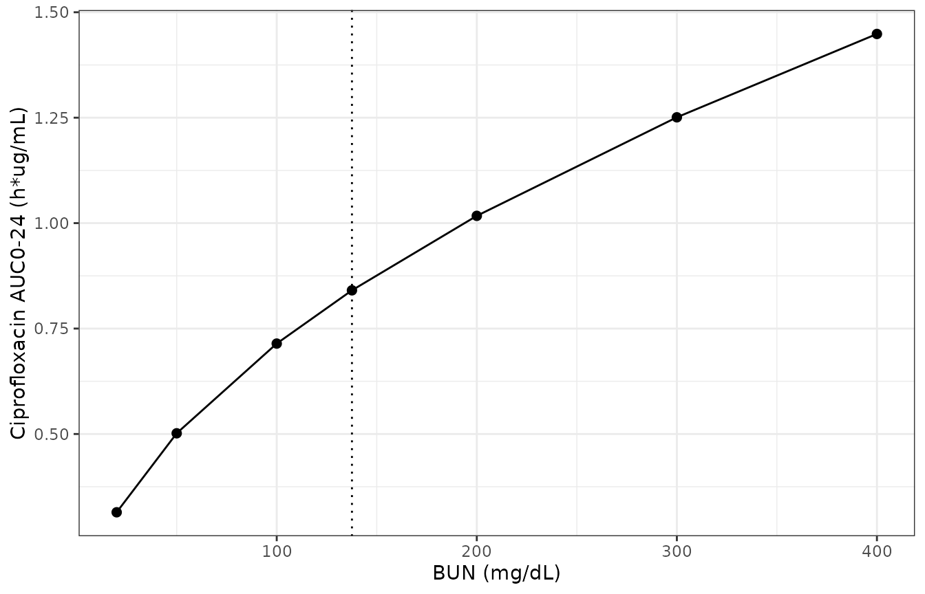
Simulated effect of BUN on ciprofloxacin exposure in the typical 3.8 kg cat, from the power effect (BUN / 137.6)^0.51 on the metabolic formation clearance.
bun_sweep |>
  transmute(
    `BUN (mg/dL)` = BUN,
    `Formation clearance (mL/h)` = cl_met,
    `Ciprofloxacin AUC0-24 (h*ug/mL)` = auc_cipro,
    `Ciprofloxacin fraction of total` = ratio
  ) |>
knitr::kable(digits = 4)| BUN (mg/dL) | Formation clearance (mL/h) | Ciprofloxacin AUC0-24 (h*ug/mL) | Ciprofloxacin fraction of total |
|---|---|---|---|
| 20.0 | 0.0486 | 0.3144 | 0.0094 |
| 50.0 | 0.0776 | 0.5017 | 0.0149 |
| 100.0 | 0.1105 | 0.7144 | 0.0211 |
| 137.6 | 0.1300 | 0.8407 | 0.0247 |
| 200.0 | 0.1573 | 1.0173 | 0.0298 |
| 300.0 | 0.1935 | 1.2509 | 0.0364 |
| 400.0 | 0.2240 | 1.4485 | 0.0419 |
Across the 20-400 mg/dL BUN range the formation clearance rises 4.6-fold and ciprofloxacin exposure rises with it, which is the direction and rough magnitude of the trend in the “nCl_EnroCipro, BUN” panel of Figure 5. Enrofloxacin exposure is essentially untouched, because the formation clearance is a negligible fraction of the parent’s total elimination (0.13 against 499.1 mL/h) – an internal inconsistency of the published parameter set that the ratio check above already exposed.
Cross-model consistency
The two models were fitted to the same cats and the same assay results, one to the summed concentration and one to the two analytes separately. Their predictions of total fluoroquinolone exposure should therefore agree.
tibble(
  Quantity = c(
    "AUC0-24 of total fluoroquinolone (h*ug/mL)",
    "Cmax of total fluoroquinolone (ug/mL)"
  ),
  `Total fluoroquinolone model` = c(
    pick("Total fluoroquinolone", "auclast"),
    pick("Total fluoroquinolone", "cmax")
  ),
  `Parent + metabolite model (sum)` = c(
    auc_enro + auc_cipro,
    max(sim_typ_met$Cc + sim_typ_met$Cc_cipro)
  )
) |>
  mutate(`% difference` = 100 *
           (`Parent + metabolite model (sum)` -
              `Total fluoroquinolone model`) /
           `Total fluoroquinolone model`) |>
knitr::kable(digits = 2)| Quantity | Total fluoroquinolone model | Parent + metabolite model (sum) | % difference |
|---|---|---|---|
| AUC0-24 of total fluoroquinolone (h*ug/mL) | 42.37 | 33.98 | -19.82 |
| Cmax of total fluoroquinolone (ug/mL) | 3.88 | 3.21 | -17.30 |
The two independent fits agree on peak concentration to within a few percent and on 0-24 h exposure to about 20%. The gap is attributable to the deep peripheral compartment of the two-compartment model (Vd2 = 2.9 x 10^4 mL with an intercompartmental clearance of 132.1 mL/h, i.e. a return half-life of about 150 h), which returns drug to plasma over the tail of the profile; the parent + metabolite model has no peripheral compartment at all. The paper itself flags Vd2 as the one parameter its bootstrap could not pin down.
Assumptions and deviations
Errata and source inconsistencies
- Volumes and clearances are labelled per kilogram but are absolute. Tables 1, 2 and 3 print “(mL/kg)” and “(mL/kg/h)”. Reading them as absolute (mL, mL/h) with the dose entered as the total amount in ug reproduces Table 1’s AUC0-24 of 46.0 h*ug/mL, the “observed clearance” median of 440.8 reported in Results 3.1, and the concentration range of Figure 1; the per-kilogram reading is four-fold low on all three. Both model files encode the absolute reading, doses are entered in ug and volumes are in mL. The arithmetic is worked through in the “Units” section above.
-
The metabolite model does not reproduce the paper’s own
ciprofloxacin:quinolone ratio. Table 1 reports that ratio as
0.18 (SE 0.02, CV% 86.39), but the formation and elimination clearances
of Table 3 imply
cl_met / cl_cipro= 0.13 / 4.6 = 0.028, i.e. about 2.5% of total fluoroquinolone on an AUC basis. The ratio depends only on those two clearances, so it cannot be reconciled by any choice of volume; a formation clearance near 1.0 mL/h would be required. The published values are encoded unchanged and the gap is quantified in the “Ciprofloxacin generation” section. Users who need a model that reproduces the 18% ratio should scalelcl_metaccordingly and document the change as their own. - The ciprofloxacin volume is not a physically possible volume. Table 3’s Vd ciprofloxacin of 22.6 mL is smaller than the plasma volume of a 4 kg cat (roughly 180 mL). It is an apparent volume that also absorbs the unidentifiable fraction of the enrofloxacin dose actually converted; the sparse three-sample design cannot separate that fraction from the formation clearance. It is encoded as published.
- Table 3 prints the formation clearance rounded to one decimal. Table 3 gives 0.1 while Table 2 gives 0.13 for the same parameter with the same SE (0.03) and the same CV% (22.9). Since 0.03 / 0.13 = 23.1% rounds to the printed 22.9% and 0.03 / 0.1 = 30.0% does not, the underlying estimate is 0.13 and that is what the model file carries.
- The Abstract is more precise than the tables for three covariate effects. The Abstract prints the weight effects on total fluoroquinolone volume and clearance as 1.63 (SE 0.19 and 0.27) and the BUN effect on metabolic formation as 0.51 (SE 0.08); Tables 1 and 3 round these to 1.6, 1.6 and 0.5. The Abstract values are used. Table 1’s CV% of 16.38 for the clearance exponent reproduces exactly as 0.27 / 1.63, confirming 1.63.
- Supplemental Table 2 reports different point estimates from Table 1. The bootstrap supplement lists “Model Estimate” values of Vd1 4793.26, Vd2 2222.57, Cl1 234.82, Cl2 190.65, dVd1weight 0.97 and dCl1weight 1.33, which differ materially from Table 1 for four of the six parameters. Table 1 is used because it is the paper’s designated final model table and because the Abstract quotes its covariate effects. The supplement appears to describe a different (probably earlier) run.
- Table 1’s CV% for Vd2 is inconsistent with its own SE. Table 1 gives Vd2 = 2.9 x 10^4 with SE 5.1 x 10^5 and CV% 17.6; 5.1e5 / 2.9e4 = 17.6 as a ratio, i.e. the true relative standard error is about 1760%, consistent with the paper’s own statement that the bootstrap could not pin this parameter down. Only the point estimate is used by the model.
-
No between-subject variance and no residual-error magnitude
are published. Methods paragraph 7 specifies exponential
inter-individual variability and a multiplicative residual model, and
Figures 2, 3 and 5 plot the empirical Bayes etas for every structural
parameter of both models, but no omega, omega-squared, SD or CV of any
random effect appears anywhere in the paper or its supplements. The CV%
columns of Tables 1-3 are relative standard errors of the typical
values. Per the standing policy for unreported variability with
structural values present, every eta and every residual SD is encoded as
fixed(0)rather than invented. Consequences: the packaged models simulate typical-value profiles only, the spread of Figure 1 cannot be reproduced, and the simulated cohort CV% of AUC0-24 is far below the published 36.33%. - AUC0-24 and “observed clearance” in Results 3.1 are on different bases. The reported group AUC0-24 medians (41.44 / 39.79 / 34.95 h*ug/mL) and clearance medians (440.8 / 365.8 / 308.5) are consistent with each other only if the clearance is Dose / AUC0-24 with the dose as the total amount – 20500 / 46.0 = 446 mL/h – and not with a per-kilogram dose. This is the same finding as erratum 1 and is what makes the units conclusion firm.
Modelling assumptions
-
Covariate functional form. Foster 2023 does not
print its covariate equations. Both covariates are encoded as powers of
the ratio to a centring value,
(WT / 3.8)^e_wt_vcand(BUN / 137.6)^e_bun_cl_met, which is Phoenix NLME’s standard continuous-covariate model and the only form consistent with the reported estimates. The centred-exponential alternative is arithmetically impossible for all three effects:exp(1.63 * (8.8 - 3.8))would multiply V1 by 3463 at the cohort’s largest cat, andexp(0.51 * (400 - 137.6))would multiply the formation clearance by 10^58 at the top of Figure 5’s BUN axis. -
BUN centring value. The paper states the weight
centring value (3.8 kg, Results 3.2) but never states one for BUN. The
cohort mean of 137.6 mg/dL is used, because the paper centres its only
other continuous covariate on the population mean. Any other centring
value rescales
lcl_metby a constant; users who prefer a different reference must rescale it accordingly. - Weight centring in the metabolite model. The 3.8 kg centring is stated only for the total fluoroquinolone model. It is applied to the metabolite model too, on the grounds that it is the same cohort, the same software and the same covariate.
-
Virtual cohort distributions. Neither the per-cat
weights nor the per-cat BUN values are published. Both are reconstructed
as log-normal quantiles matched to the published marginal summaries,
deterministically (via
ppoints()) so the vignette is reproducible without a seed. They control the only between-cat variability in the simulations. -
Infusion duration. Doses are given as 30-minute
infusions (
rate = amt / 0.5), matching Methods paragraph 3. The paper does not say whether the fit treated the dose as an infusion or a bolus; over a profile with an 8-hour half-life the difference is negligible after the first hour. -
Renal function is deliberately absent from both
models. Serum creatinine, SDMA and (for the total
fluoroquinolone model) BUN were screened and dropped. They are recorded
in each model’s
covariatesDataExcludedmetadata so the screen is auditable, and no effect is encoded. This absence is the paper’s principal finding, not an omission. - Cohort size. 34 cats, matching the study, well under the 200-per-arm vignette cap.