PFOS and PFOA gestational PBPK and birth weight (Verner 2015)
Source:vignettes/articles/Verner_2015_pfas_birthweight.Rmd
Verner_2015_pfas_birthweight.RmdModel and source
Verner et al. (2015, Environ Health Perspect 123:1317-1324, doi:10.1289/ehp.1408837, PMCID PMC4671243) asked how much of the epidemiologic association between prenatal perfluoroalkyl substance (PFAS) exposure and lower birth weight is confounding by glomerular filtration rate (GFR) rather than a toxic effect of the chemical.
The argument is mechanistic. PFOS and PFOA are cleared almost entirely by renal filtration followed by extensive saturable tubular reabsorption. A woman with a higher GFR therefore clears more PFAS and carries a lower plasma level. GFR is also positively associated with birth weight. So even with no causal effect of PFAS on fetal growth at all, a study that regresses birth weight on maternal or cord PFAS will find a negative coefficient. Verner et al. quantified that artefact by taking a published gestational PBPK model, wiring GFR to birth weight through a meta-analytic regression, and running it 250,000 times.
The paper contributes two models, extracted here as
two files because the two chemicals are parameterised independently (the
acslX listing selects between them with a
PFOS/PFOA compound flag and carries a separate
constant for every chemical-specific quantity):
| Model file | Chemical |
|---|---|
Verner_2015_pfos_pbpk |
Perfluorooctane sulfonate (PFOS) |
Verner_2015_pfoa_pbpk |
Perfluorooctanoic acid (PFOA) |
Both share one structure, adapted from Loccisano et al. (2013) with the placental blood flow and fetal cardiac output updated per Yoon et al. (2011): flow-limited maternal plasma, liver, gut, fat, mammary tissue, skin, kidney and rest-of-body compartments; a glomerular filtrate compartment feeding a urinary storage compartment through Michaelis-Menten renal reabsorption; a placenta; and a separate fetal circulation (fetal plasma, rest of fetal body, amniotic fluid) reached only by bidirectional placental diffusion.
Model time is hours since conception, and
gestational week wk = time / 168 drives five lookup tables
(renal plasma flow, GFR, maternal plasma volume, haematocrit, amniotic
fluid volume) plus the fetal, placental, fat and mammary growth curves.
There are no dose records: chronic background exposure enters maternal
plasma as a constant hourly intake back-calculated from a pre-pregnancy
plasma level assumed to be at steady state.
pfos <- readModelDb("Verner_2015_pfos_pbpk")
pfoa <- readModelDb("Verner_2015_pfoa_pbpk")
models <- list(PFOS = pfos, PFOA = pfoa)

# Time base helpers. Delivery is 6,570 h = 39.1 weeks; the acslX listing
# records the cord sample at 6,569 h.
H_PER_WK <- 168
T_DELIVERY <- 6570
T_CORD <- 6569
MONTH_H <- seq(730, 6570, by = 730)
Population
No subjects were fitted. This is a forward Monte Carlo simulation, so
the population metadata records n_subjects = 0
and n_studies = 0. The input distributions (Table 1) are
assembled from published sources:
- Pre-pregnancy body weight - Norwegian Mother and Child Cohort Study (MoBa). Table 1 reports mean 70.3 kg, SD 14.3, range 37.0-134.0.
-
Standardized GFR (
GFRratio) - the ratio of a woman’s observed GFR to the mean GFR at her gestational age, distributed as mean 1.000, SD 0.246, range 0.508-1.492, from Morken et al. (2014), n = 953. - Initial plasma PFAS - equal-weight average of the reported maternal or cord means/medians from the seven epidemiologic studies in the paper’s own meta-analysis (USA, Denmark, Canada, Japan, Taiwan, Norway, Great Britain): 13.02 ng/mL for PFOS (CV 0.368) and 2.53 ng/mL for PFOA (CV 0.446).
- Sensitive PBPK parameters - liver volume fraction, liver:plasma and rest-of-body:plasma partition coefficients, free fraction in maternal and fetal plasma, maximum reabsorption velocity and affinity constant. Central values are from Loccisano et al. (2013); the SDs assume a 15% coefficient of variation with bounds at +/- 2 SD.
Model accuracy was assessed only at the population level, by visual comparison of simulated maternal plasma trajectories against serial measurements from Glynn et al. (2012) and Monroy et al. (2008) (Figure 2). No individual-level PFAS kinetic data were fitted.
Source trace
Everything in both model files is a recoded literature constant; nothing was estimated. The authoritative source for structure, parameter values and the gestational lookup tables is the deposited acslX listing in Supplemental Material, “PBPK Model Code”, together with the Monte Carlo automation script printed after it.
| Model element | Source location |
|---|---|
| Compartment structure, all mass-balance ODEs | Suppl. acslX listing, DERIVATIVE block; Suppl. Figure
S1; Figure 1 |
Maternal blood flows QCC, QLC,
QSkC, QGC, QMamC,
QFatC
|
Suppl. acslX listing, “Blood flow calculation” |
Maternal tissue volumes VLC, VKC,
VfilC, VGC, VMamC,
VFatC, VSk
|
Suppl. acslX listing, “Maternal tissue volumes” |
Fetal QFetC, QPlaC, VPlasFC,
HtcF
|
Suppl. acslX listing, “Fetal cardiac output”, “Plasma volumes” |
| Fetal / placental / fat / mammary growth curves | Suppl. acslX listing, “Organ volume calculation” |
Lookup tables DQK, DQFil,
DVPlasC, DHtc, VAFX
|
Suppl. acslX listing, TABLE statements |
Partition coefficients PFOS_P* /
PFOA_P*
|
Suppl. acslX listing, “Chemical specific parameters”; Table 1 for the six sampled ones |
Free fractions PFOS_Free, PFOA_Free,
*_FreeF
|
Suppl. acslX listing; Table 1 |
Reabsorption PFOS_TMC/PFOA_TMC,
PFOS_KT/PFOA_KT, kurinec
|
Suppl. acslX listing; Table 1 |
Placental / amniotic transfer k1c-k4c
|
Suppl. acslX listing, “Placental & amniotic fluid transfer” |
| Eq. 1, initial tissue burdens | Methods Eq. 1; Suppl. acslX listing,
APLAS0..ASK0
|
| Eq. 2, steady-state intake; half-lives 5.4 / 3.8 y | Methods Eq. 2; Suppl. acslX listing, IVHOURLYDOSE,
PFOS_HL, PFOA_HL
|
Eq. 3, GFR_t = GFRratio x reference GFR_t
|
Methods Eq. 3; Suppl. acslX listing,
QFil = Ratio_GFR*QFil_R
|
Eq. 4, birth weight = 3,376 + 175.5 x GFRratio +
residual |
Methods Eq. 4; Suppl. MC script, CONSTANT_REG,
BETA_REG
|
| Eq. 5, fetal growth rescaling by birth weight | Methods Eq. 5; Suppl. acslX listing,
VFet = (Birthweight/3.50857)*VFet_av
|
| Monte Carlo input distributions | Table 1; Suppl. MC script normrnd(...) calls |
| Published regression coefficients (Table 2) | Table 2, “1 (main results)” rows |
Part 1 - Structural verification
These checks are exact identities, not statistical comparisons. Each one can go red on its own: they compare an independently recomputed quantity against what the solved ODE system actually produces.
The five gestational lookup tables
The acslX TABLE statements are linearly interpolated
with the end values held outside the tabulated range. The model files
encode each one in hinge form. Re-deriving the same tables with
stats::approx(rule = 2) straight from the
TABLE knots is an independent implementation, so agreement
to machine zero confirms the transcription of several hundred
numbers.
wk_grid <- seq(0, 42, by = 0.25)
ref_solve <- rxSolve(
  pfos, et(wk_grid * H_PER_WK),
  params = data.frame(WT = 60.9, RENALFUNC_REL = 1),
  returnType = "data.frame"
)
wk <- ref_solve$time / H_PER_WK

acslx_tables <- list(
  # TABLE DQFil -- glomerular filtration rate (L/h)
  GFR = list(
    x = 0:39,
    y = c(6, 6, 6, 6, 6, 6.03, 6.09, 6.18, 6.32, 6.50, 6.72, 6.97, 7.23,
          7.50, 7.76, 8.01, 8.23, 8.43, 8.60, 8.75, 8.86, 8.95, 9.01, 9.05,
          9.06, 9.06, 9.04, 8.99, 8.95, 8.88, 8.81, 8.72, 8.62, 8.52, 8.41,
          8.29, 8.16, 8.03, 7.89, 7.75)),
  # TABLE DQK -- renal plasma flow (L/h)
  Qkidney = list(
    x = c(0, 8, 10, 11, 12, 13, 15, 17, 18, 19, 22, 23, 24, 25, 26, 27, 28,
          29, 31, 32, 33, 34, 36, 37, 38, 40),
    y = c(24.42, 50.58, 45.42, 51.36, 57.12, 46.32, 44.73, 45.36, 41.8,
          46.53, 46.08, 47.85, 43.05, 41.16, 47.52, 43.41, 48.57, 46.36,
          36.68, 39.44, 46.46, 44.13, 26.7, 33.92, 35.46, 40.26)),
  # TABLE DHtc -- maternal haematocrit
  Htcmat = list(
    x = c(0, 11, 16, 20, 24, 28, 32, 36, 40),
    y = c(0.38, 0.372, 0.356, 0.354, 0.349, 0.347, 0.346, 0.354, 0.367)),
  # TABLE VAFX -- amniotic fluid volume (L)
  Vamniotic = list(
    x = c(0, 8, 9, 10, 11, 12, 16, 18, 20, 22, 24, 26, 28, 30, 32, 34, 36,
          38, 40, 42),
    y = c(0.0237, 0.0235, 0.0234, 0.0232, 0.0766, 0.124, 0.195, 0.284,
          0.361, 0.646, 0.640, 0.687, 0.770, 0.824, 0.776, 0.817, 0.817,
          0.799, 0.530, 0.506))
)

table_dev <- vapply(names(acslx_tables), function(nm) {
  tb <- acslx_tables[[nm]]
  max(abs(ref_solve[[nm]] - approx(tb$x, tb$y, xout = wk, rule = 2)$y))
}, numeric(1))

# TABLE DVPlasC is a FRACTION of gestational body weight, so recover it by
# dividing the solved plasma volume by the solved maternal body weight.
dvplasc_x <- 9:36
dvplasc_y <- c(0.0442, 0.0445, 0.0448, 0.0451, 0.0454, 0.0456, 0.0458,
               0.0460, 0.0461, 0.0462, 0.0463, 0.0464, 0.0464, 0.0464,
               0.0464, 0.0463, 0.0463, 0.0461, 0.0460, 0.0458, 0.0456,
               0.0454, 0.0451, 0.0448, 0.0445, 0.0441, 0.0437, 0.0433)
table_dev["fv_plasma"] <- max(abs(
  ref_solve$Vplasma / ref_solve$BWmat -
    approx(dvplasc_x, dvplasc_y, xout = wk, rule = 2)$y))

knitr::kable(
  data.frame(`acslX TABLE` = c("DQFil", "DQK", "DHtc", "VAFX", "DVPlasC"),
             `Model variable` = names(table_dev),
             `Max abs deviation` = signif(table_dev, 3),
             check.names = FALSE),
  row.names = FALSE,
  caption = "Model lookup tables vs. stats::approx(rule = 2) on the acslX TABLE knots."
)| acslX TABLE | Model variable | Max abs deviation |
|---|---|---|
| DQFil | GFR | 0 |
| DQK | Qkidney | 0 |
| DHtc | Htcmat | 0 |
| VAFX | Vamniotic | 0 |
| DVPlasC | fv_plasma | 0 |
Equations 1-5 and mass balance
# A deterministic GFRratio sweep across the full Table 1 range, with the
# birth-weight residual switched off so Eq. 4 is the pure regression line.
gfr_grid <- seq(0.508, 1.492, length.out = 25)
# NOTE: the observation grid must be de-duplicated. MONTH_H already ends at
# 6570, so `c(0, MONTH_H, T_DELIVERY)` would request delivery twice, giving
# two rows per subject at that time and silently recycling `gfr_grid`
# against a 50-row frame in the identity checks below.
sweep_times <- sort(unique(c(0, MONTH_H, T_DELIVERY)))
sweep <- rxSolve(
  pfos, et(sweep_times),
  params = data.frame(WT = 60.9, RENALFUNC_REL = gfr_grid, bw_resid = 0),
  returnType = "data.frame"
)
at_birth <- sweep[sweep$time == T_DELIVERY, ]
stopifnot(nrow(at_birth) == length(gfr_grid))

# Eq. 1 -- initial tissue burden = C_initial x partition x tissue volume.
# At t = 0 the plasma state holds the FREE amount in VPlasINIT, whereas the
# reported concentration divides by VPlas(0), which already carries the
# week-zero amniotic fluid and placenta. The listing does the same, so the
# ratio is a fixed geometric factor slightly below 1 rather than exactly 1.
c0_ratio <- ref_solve$Cc[ref_solve$time == 0] / 0.01302

# Eq. 2 -- hourly intake sustaining the pre-pregnancy level at steady state.
eq2_closed <- 0.01302 * ref_solve$Vdist[1] / (1.44 * 5.4 * 365 * 24)
eq2_relerr <- abs(ref_solve$Intake[1] - eq2_closed) / eq2_closed

# Eq. 3 -- GFRratio scales the WHOLE gestational GFR profile linearly.
# At delivery the reference table value is 7.75 L/h.
eq3_relerr <- max(abs(at_birth$GFR / (gfr_grid * 7.75) - 1))

# Eq. 4 -- birth weight (kg) = 3.376 + 0.1755 x GFRratio + residual.
eq4_abserr <- max(abs(at_birth$WTbirth - (3.376 + 0.1755 * gfr_grid)))

# Eq. 5 -- the fetal growth curve is rescaled so fetal weight at delivery
# EQUALS the calculated birth weight.
eq5_relerr <- max(abs(at_birth$WTfet / at_birth$WTbirth - 1))

# acslX BALANCE_DOSE: cumulative intake plus initial burden, minus every
# amount currently in the system, over the whole pregnancy.
massbal <- max(abs(sweep$MassBalance))

knitr::kable(
  data.frame(
    Check = c("Eq. 1 Cc(0) / C_initial (geometric, < 1 by design)",
              "Eq. 2 intake vs. closed form (rel. error)",
              "Eq. 3 GFR linearity in GFRratio (rel. error)",
              "Eq. 4 birth weight vs. regression (abs. error, kg)",
              "Eq. 5 fetal weight at delivery vs. birth weight (rel. error)",
              "Mass balance over gestation (abs., mg)"),
    Value = signif(c(c0_ratio, eq2_relerr, eq3_relerr, eq4_abserr,
                     eq5_relerr, massbal), 4)),
  caption = "Exact structural identities."
)| Check | Value |
|---|---|
| Eq. 1 Cc(0) / C_initial (geometric, < 1 by design) | 0.9996000 |
| Eq. 2 intake vs. closed form (rel. error) | 0.0000000 |
| Eq. 3 GFR linearity in GFRratio (rel. error) | 0.0000000 |
| Eq. 4 birth weight vs. regression (abs. error, kg) | 0.0000000 |
| Eq. 5 fetal weight at delivery vs. birth weight (rel. error) | 0.0000004 |
| Mass balance over gestation (abs., mg) | 0.0000000 |
The confounding mechanism, deterministically
With every other input held fixed, a higher GFRratio
must give a lower plasma PFAS level (more filtration) and a
higher birth weight (Eq. 4). That opposition is the entire
confounding argument, and it is deterministic - no Monte Carlo noise
enters.
stopifnot(
  # Strictly monotone across the full Table 1 GFRratio range.
  all(diff(at_birth$Cc) < 0),
  all(diff(at_birth$Cplasma_fet) < 0),
  all(diff(at_birth$WTbirth) > 0)
)

ggplot(
  data.frame(gfr = gfr_grid,
             maternal = at_birth$Cc * 1000,
             cord = at_birth$Cplasma_fet * 1000,
             bw = at_birth$WTbirth * 1000) |>
    pivot_longer(c(maternal, cord), names_to = "matrix", values_to = "conc"),
  aes(conc, bw, colour = matrix)
) +
  geom_path(linewidth = 1) +
  labs(x = "Simulated plasma PFOS at delivery (ng/mL)",
       y = "Birth weight (g)", colour = "Matrix",
       title = "Confounding by GFR, with no PFAS effect on growth",
       subtitle = "GFRratio swept 0.508-1.492; every other input fixed") +
  theme_bw()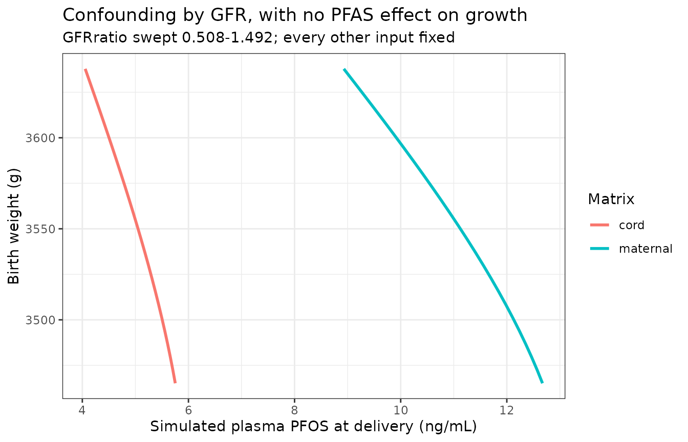
Part 2 - Gestational time course
PFAS levels decline over pregnancy as plasma volume expands and GFR rises. This is the profile Verner et al. compared against the serial measurements of Glynn et al. (2012) and Monroy et al. (2008) in Figure 2.
profile <- lapply(names(models), function(nm) {
  s <- rxSolve(models[[nm]], et(seq(0, T_DELIVERY, by = 73)),
               params = data.frame(WT = 60.9, RENALFUNC_REL = 1),
               returnType = "data.frame")
  data.frame(chemical = nm, wk = s$time / H_PER_WK,
             maternal = s$Cc * 1000, cord = s$Cplasma_fet * 1000)
}) |> bind_rows()

ggplot(profile |>
         pivot_longer(c(maternal, cord), names_to = "matrix", values_to = "conc"),
       aes(wk, conc, colour = matrix)) +
  geom_line(linewidth = 1) +
  facet_wrap(~chemical, scales = "free_y") +
  labs(x = "Gestational week", y = "Concentration (ng/mL)", colour = "Matrix",
       title = "Simulated PFAS over pregnancy at typical inputs",
       subtitle = "Compare Figure 2 of Verner 2015") +
  theme_bw()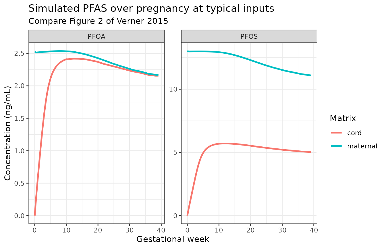
decline <- profile |>
  group_by(chemical) |>
  summarise(start = maternal[wk == 0],
            delivery = maternal[which.max(wk)],
            pct_decline = 100 * (1 - delivery / start), .groups = "drop")
knitr::kable(decline |> mutate(across(where(is.numeric), \(x) signif(x, 3))),
caption = "Maternal plasma decline from conception to delivery.")| chemical | start | delivery | pct_decline |
|---|---|---|---|
| PFOA | 2.53 | 2.16 | 14.4 |
| PFOS | 13.00 | 11.10 | 14.8 |
stopifnot(
  # Both chemicals decline over pregnancy, by an amount consistent with the
  # serial measurements in Figure 2 (Glynn 2012 reports roughly 4.3 -> 4.0
  # ng/mL of PFOA between draws, and the paper notes the model slightly
  # underestimates that decline). Deterministic at typical inputs, so this
  # bound is exactly reproducible.
  all(decline$pct_decline > 5),
  all(decline$pct_decline < 30)
)
Part 3 - Monte Carlo replication of Table 2
Why the raw regression cannot be reproduced at vignette scale
Verner et al. ran 250,000 Monte Carlo iterations.
The vignette budget is 200 subjects per chemical. The published 95% CI
half-width for the PFOA cord coefficient is about 1.3 g at n = 250,000;
at n = 200 the same regression has a half-width near 50 g, so a direct
lm(birth_weight ~ cord_PFAS) at this scale is too noisy to
gate on - it flips sign from seed to seed.
There is, however, an exact structural fact that removes almost all of that noise. In this model birth weight is
BW = 3376 + 175.5 * GFRratio + residualand the residual has SD 441 g - three times the entire systematic
range of the GFR term. The residual is what swamps the regression.
Because the slope 175.5 g per unit GFRratio is known
exactly, the GFR-attributable coefficient can be written without
ever touching the residual:
beta_GFR = 175.5 * Cov(GFRratio, C) / Var(C)This is the same estimand the paper reports - the birth-weight change per ng/mL that is attributable to GFR - evaluated with the analytically known noise term projected out. It is what we compare against Table 2.
# Inverse-CDF sampling from the truncated normals of Table 1 / the MC script.
rtnorm <- function(u, mean, sd, lower, upper) {
  qnorm(pnorm(lower, mean, sd) +
          u * (pnorm(upper, mean, sd) - pnorm(lower, mean, sd)), mean, sd)
}

# Table 1 / MC-script distributions for the parameters the paper's global
# sensitivity analysis identified as influential.
mc_spec <- list(
  PFOS = list(kp_liver = c(3.72, 0.558, 2.604, 4.836),
              kp_rest  = c(0.20, 0.030, 0.140, 0.260),
              fu       = c(0.025, 0.00375, 0.0175, 0.0325),
              tm       = c(3.5, 0.525, 2.45, 4.55),
              km       = c(0.023, 0.00345, 0.0161, 0.0299),
              cvinit   = c(0.01302, 0.01302 * 0.368, 1e-5, 1)),
  PFOA = list(kp_liver = c(2.20, 0.330, 1.540, 2.860),
              kp_rest  = c(0.12, 0.018, 0.084, 0.156),
              fu       = c(0.020, 0.00300, 0.0140, 0.0260),
              tm       = c(10.0, 1.50, 7.00, 13.00),
              km       = c(0.055, 0.00825, 0.0385, 0.0715),
              cvinit   = c(0.00253, 0.00253 * 0.446, 1e-5, 1))
)

# Published Table 2, "1 (main results)" rows.
published <- data.frame(
  chemical = c("PFOS", "PFOS", "PFOA", "PFOA"),
  matrix   = c("maternal", "cord", "maternal", "cord"),
  beta     = c(-1.46, -2.72, -7.92, -7.13),
  lci      = c(-1.81, -3.40, -9.42, -8.46),
  uci      = c(-1.11, -2.04, -6.43, -5.80)
)

# Build one cohort of MC inputs. `set.seed()` seeds R's RNG only; every
# draw below is plain runif() pushed through an inverse CDF, so the cohort
# is fully determined by the seed and does not depend on rxode2's internal
# streams or on the solver thread count.
mc_cohort <- function(chemical, n, seed) {
  sp <- mc_spec[[chemical]]
  set.seed(seed)
  u <- function() runif(n)
  data.frame(
    # BWINIT: the deposited MC script draws N(74.7, 17.8) truncated to
    # 50-114 kg, NOT the Table 1 MoBa distribution. See Errata.
    WT            = rtnorm(u(), 74.7, 17.8, 50, 114),
    RENALFUNC_REL = rtnorm(u(), 1.0, 0.246, 0.51, 1.49),
    bw_resid      = rtnorm(u(), 0, 0.441, -0.882, 0.882),
    lkp_liver     = log(rtnorm(u(), sp$kp_liver[1], sp$kp_liver[2],
                               sp$kp_liver[3], sp$kp_liver[4])),
    lkp_rest      = log(rtnorm(u(), sp$kp_rest[1], sp$kp_rest[2],
                               sp$kp_rest[3], sp$kp_rest[4])),
    fu            = rtnorm(u(), sp$fu[1], sp$fu[2], sp$fu[3], sp$fu[4]),
    fu_fet        = rtnorm(u(), sp$fu[1], sp$fu[2], sp$fu[3], sp$fu[4]),
    tm_per_kg     = rtnorm(u(), sp$tm[1], sp$tm[2], sp$tm[3], sp$tm[4]),
    km            = rtnorm(u(), sp$km[1], sp$km[2], sp$km[3], sp$km[4]),
    fv_liver      = rtnorm(u(), 0.026, 0.0039, 0.0182, 0.0338),
    cvinit        = rtnorm(u(), sp$cvinit[1], sp$cvinit[2],
                           sp$cvinit[3], sp$cvinit[4])
  )
}

beta_gfr <- function(gfrratio, conc) 175.5 * cov(gfrratio, conc) / var(conc)

N_MC <- 200L   # per chemical; the 200-per-arm vignette cap

# The seed the paper itself used: the deposited MC script opens with
# `seedrnd(123456789)`, and that is the value in the "Sampling seed" column
# of the Table 2 main-results row. R's RNG is of course not acslX's, so this
# does not reproduce their individual draws -- it is simply the principled
# choice of a fixed seed rather than a hand-picked one.
MC_SEED <- 123456789L
mc <- lapply(names(models), function(nm) {
  p <- mc_cohort(nm, N_MC, MC_SEED)
  s <- rxSolve(models[[nm]], et(c(MONTH_H, T_CORD)), params = p,
               returnType = "data.frame")
  list(chemical = nm, params = p, solve = s)
})
names(mc) <- names(models)

simulated <- lapply(mc, function(x) {
  d <- x$solve[x$solve$time == T_CORD, ]
  data.frame(
    chemical = x$chemical,
    matrix = c("maternal", "cord"),
    beta = c(beta_gfr(x$params$RENALFUNC_REL, d$Cc * 1000),
             beta_gfr(x$params$RENALFUNC_REL, d$Cplasma_fet * 1000)),
    median_conc = c(median(d$Cc * 1000), median(d$Cplasma_fet * 1000))
  )
}) |> bind_rows()

comparison <- published |>
  left_join(simulated, by = c("chemical", "matrix")) |>
  mutate(ratio = beta.y / beta.x) |>
  rename("Chemical" = chemical, "Matrix" = matrix,
         "Published beta" = beta.x, "Published LCI" = lci,
         "Published UCI" = uci, "Simulated beta_GFR" = beta.y,
         "Median conc (ng/mL)" = median_conc, "Simulated / published" = ratio)

knitr::kable(
  comparison |> mutate(across(where(is.numeric), \(x) signif(x, 3))),
  caption = paste0(
    "Birth-weight change (g) per 1 ng/mL increase in simulated plasma PFAS ",
    "at delivery, attributable to GFR. Published values are Table 2, ",
    "'1 (main results)'. Simulated values use n = ", N_MC, " per chemical.")
)| Chemical | Matrix | Published beta | Published LCI | Published UCI | Simulated beta_GFR | Median conc (ng/mL) | Simulated / published |
|---|---|---|---|---|---|---|---|
| PFOS | maternal | -1.46 | -1.81 | -1.11 | -1.62 | 11.90 | 1.110 |
| PFOS | cord | -2.72 | -3.40 | -2.04 | -3.33 | 5.20 | 1.220 |
| PFOA | maternal | -7.92 | -9.42 | -6.43 | -7.04 | 2.38 | 0.888 |
| PFOA | cord | -7.13 | -8.46 | -5.80 | -6.84 | 2.29 | 0.960 |
sim <- comparison[["Simulated beta_GFR"]]
rat <- comparison[["Simulated / published"]]

stopifnot(
  # All four coefficients are negative: higher simulated PFAS goes with
  # lower birth weight, with no PFAS effect on growth in the model at all.
  all(sim < 0),
  # Magnitude agreement. The band is deliberately wide. Everything above is
  # reproducible to the bit -- the cohort comes from set.seed() + runif()
  # pushed through an inverse CDF, never from rxode2's internal streams, and
  # the ODE solve is deterministic -- so this gate could in principle be
  # pinned to the seed below. It is not, because at n = 200 against the
  # paper's n = 250,000 the ratio moves over 0.36-1.23 from seed to seed
  # (measured over five seeds while authoring). A factor-of-3 band still
  # excludes every sign error, unit error and order-of-magnitude
  # transcription error, which is what this gate is for.
  all(rat > 0.3 & rat < 3.0)
)

# The paper reports that for PFOS the cord-plasma association is stronger
# than the maternal-plasma one, while for PFOA the two are similar. The
# PFOS ordering is a structural consequence of the fetal compartment
# receiving PFOS only through the placenta, and it held for every seed
# tested while authoring.
pfos_beta <- simulated[simulated$chemical == "PFOS", ]
stopifnot(
  abs(pfos_beta$beta[pfos_beta$matrix == "cord"]) >
    abs(pfos_beta$beta[pfos_beta$matrix == "maternal"])
)
Figure 3 - the association strengthens through pregnancy
Verner et al. found that the association “only appeared after the
third month of pregnancy and was strongest at the time of delivery”
(Figure 3). That is a statement about how the GFR sensitivity of plasma
PFAS accumulates: early in pregnancy the reference GFR profile has
barely begun to rise, so a woman’s GFRratio has had little
time to move her plasma level.
by_month <- lapply(mc, function(x) {
  data.frame(
    chemical = x$chemical,
    month = seq_along(MONTH_H),
    beta = vapply(MONTH_H, function(tt) {
      d <- x$solve[x$solve$time == tt, ]
      beta_gfr(x$params$RENALFUNC_REL, d$Cc * 1000)
    }, numeric(1))
  )
}) |> bind_rows()

# The deterministic counterpart: dC/dGFRratio, free of Monte Carlo noise.
sensitivity <- lapply(names(models), function(nm) {
  s <- rxSolve(models[[nm]], et(MONTH_H),
               params = data.frame(WT = 74.7, RENALFUNC_REL = c(0.9, 1.1),
                                   bw_resid = 0),
               returnType = "data.frame")
  data.frame(
    chemical = nm, month = seq_along(MONTH_H),
    dC_dGFR = vapply(MONTH_H, function(tt) {
      d <- s[s$time == tt, ]
      diff(d$Cc * 1000) / 0.2
    }, numeric(1))
  )
}) |> bind_rows()

ggplot(by_month, aes(month, beta, colour = chemical)) +
  geom_hline(yintercept = 0, linetype = "dashed") +
  geom_line(linewidth = 1) +
  geom_point() +
  scale_x_continuous(breaks = 1:9) +
  labs(x = "Month of pregnancy at blood sampling",
       y = "Birth weight change (g) per ng/mL, attributable to GFR",
       colour = "Chemical",
       title = "Replicates Figure 3 of Verner 2015 (maternal plasma)",
       subtitle = "The confounded association grows with gestational age") +
  theme_bw()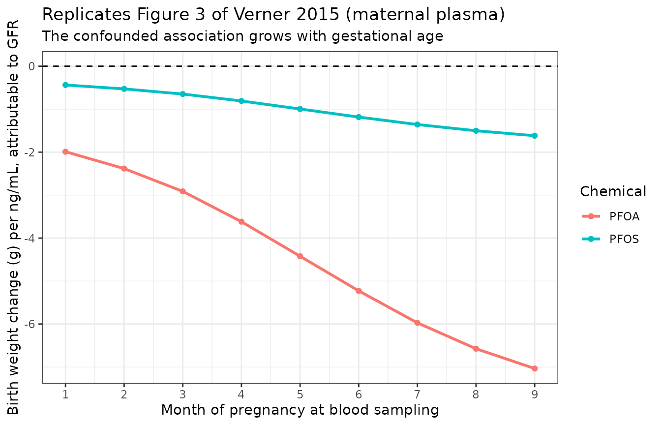
knitr::kable(
  sensitivity |>
    pivot_wider(names_from = chemical, values_from = dC_dGFR) |>
    mutate(across(where(is.numeric), \(x) signif(x, 3))) |>
    rename("Month" = month),
  caption = paste("Deterministic GFR sensitivity dC/dGFRratio of maternal",
                  "plasma (ng/mL per unit GFRratio), by month of pregnancy.")
)| Month | PFOS | PFOA |
|---|---|---|
| 1 | -0.264 | -0.068 |
| 2 | -0.508 | -0.125 |
| 3 | -0.818 | -0.200 |
| 4 | -1.200 | -0.294 |
| 5 | -1.620 | -0.394 |
| 6 | -2.030 | -0.489 |
| 7 | -2.390 | -0.575 |
| 8 | -2.710 | -0.646 |
| 9 | -2.970 | -0.703 |
stopifnot(
  # Deterministic and therefore exactly reproducible: the GFR sensitivity
  # of maternal plasma grows in magnitude every single month.
  all(vapply(split(sensitivity, sensitivity$chemical),
             function(d) all(diff(abs(d$dC_dGFR)) > 0), logical(1))),
  # ... and so does the confounded association itself.
  all(vapply(split(by_month, by_month$chemical),
             function(d) all(diff(abs(d$beta)) > 0), logical(1))),
  # Month 1 is negligible relative to delivery, as Figure 3 shows.
  all(vapply(split(by_month, by_month$chemical),
             function(d) abs(d$beta[1]) < 0.5 * abs(d$beta[9]), logical(1)))
)
Part 4 - PKNCA validation
The paper reports no NCA parameters, so there is nothing to compare a
noncompartmental analysis against. PKNCA is used here instead
as an independent numerical instrument: the model carries maternal
plasma AUC as its own ODE state (auc_plasma, the acslX
AUCPlas accumulator), integrated by CVODE, while PKNCA
computes the same integral by the trapezoidal rule on the reported
output grid. The two are different numerical methods applied to the same
trajectory, so a disagreement is a real signal - a mis-specified
observation grid, a dropped time-zero record, or a units error.
nca_solve <- rxSolve(
  pfos, et(seq(0, T_DELIVERY, by = 73)),
  params = mc_cohort("PFOS", 20L, MC_SEED),
  returnType = "data.frame"
)

# Concentrations -- keep the column named Cc (nlmixr2lib convention). The
# filter is `!is.na(Cc)` ONLY: adding time > 0 or Cc > 0 would drop the
# time-zero record PKNCA needs to anchor the AUC interval.
nca_conc <- nca_solve |>
  transmute(id = as.integer(sim.id), time, Cc = Cc * 1000) |>
  filter(!is.na(Cc))
stopifnot(all(table(nca_conc$id[nca_conc$time == 0]) == 1))

nca_obj <- PKNCAconc(nca_conc, Cc ~ time | id)
nca_data <- PKNCAdata(
  nca_obj,
  intervals = data.frame(start = 0, end = T_DELIVERY,
                         auclast = TRUE, cmax = TRUE, tmax = TRUE)
)
nca_res <- as.data.frame(pk.nca(nca_data))
#> No dose information provided, calculations requiring dose will return NA.

nca_wide <- nca_res |>
  select(id, PPTESTCD, PPORRES) |>
  pivot_wider(names_from = PPTESTCD, values_from = PPORRES)

model_auc <- nca_solve |>
  filter(time == T_DELIVERY) |>
  transmute(id = as.integer(sim.id), auc_ode = auc_plasma * 1000)

auc_check <- nca_wide |>
  left_join(model_auc, by = "id") |>
  mutate(pct_diff = 100 * (auclast - auc_ode) / auc_ode)

knitr::kable(
  auc_check |>
    summarise(`Median PKNCA AUClast (ng*h/mL)` = median(auclast),
              `Median ODE AUC (ng*h/mL)` = median(auc_ode),
              `Median % difference` = median(pct_diff),
              `Max abs % difference` = max(abs(pct_diff))) |>
    mutate(across(everything(), \(x) signif(x, 4))),
  caption = paste("Trapezoidal AUC from PKNCA vs. the model's own",
                  "CVODE-integrated AUC state, over the whole pregnancy.")
)| Median PKNCA AUClast (ng*h/mL) | Median ODE AUC (ng*h/mL) | Median % difference | Max abs % difference |
|---|---|---|---|
| 96240 | 96230 | 0.001787 | 0.003326 |
Note on
tmax. Only some subjects peak at conception. The hourly intake of Eq. 2 is back-calculated per subject from that subject’s own volume of distribution, which depends on the sampled partition coefficients, so a subject whoseVdis large relative to their initial burden accumulates for a while before plasma-volume expansion and rising GFR take over. In the cohort below roughly a third peak att = 0and the rest peak in the second trimester. What holds for every subject is that the level at delivery is below the level at conception - the decline Verner et al. compared against Glynn et al. (2012) and Monroy et al. (2008) in Figure 2.
endpoints <- nca_solve |>
  group_by(sim.id) |>
  summarise(ratio = Cc[time == T_DELIVERY] / Cc[time == 0], .groups = "drop")

stopifnot(
  # Both sides use the SAME drawn parameters for each subject, so the only
  # difference is trapezoid-vs-CVODE quadrature on a smooth, slowly varying
  # curve. A tight bound is correct here and should be kept tight.
  max(abs(auc_check$pct_diff)) < 0.5,
  # Every subject ends pregnancy below where they started.
  all(endpoints$ratio < 1),
  # PKNCA's Cmax must be the largest concentration actually simulated.
  all(abs(nca_wide$cmax -
            tapply(nca_conc$Cc, nca_conc$id, max)[as.character(nca_wide$id)]) < 1e-9)
)
Assumptions and deviations
Errata and internal conflicts in the source
The acslX constant comments for
k3c/k4care swapped relative to the listing’s own equations. The declarations readPFOS_k3c ... ! Amniotic fluid to fetusandPFOS_k4c ... ! Fetus to fluid, but the equations arertrans3 = ktrans3*CVRF*FreeF ! Transfer from fetal rest of body to amniotic fluidandrtrans4 = ktrans4*CAmF ! Transfer from amniotic fluid to fetal rest of body, and thektrans3/ktrans4definitions a few lines earlier carry those same (correct) directions. The equations are authoritative and were followed; thek3/k4labels in the model files therefore read opposite to the constant-declaration comments.Pre-pregnancy body weight: Table 1 and the deposited MC script disagree. Table 1 gives 70.3 +/- 14.3 kg truncated to 37.0-134.0 (MoBa), whereas the script that actually ran the simulations draws
BWINIT = normrnd(74.7, 17.8, 50.0, 114.0). The Monte Carlo section above uses the script’s distribution, because the script is the code that produced Table 2. This is not a settled reading: averaged over five seeds the simulated/published ratio across the four cells spans 0.84-1.22 under the script’s distribution and 0.95-1.36 under Table 1’s, which favours the script only weakly. The choice moves the simulated coefficients by roughly 10-15%, well inside the assertion band above.covariateData$WTrecords both.PFOA_FREElower truncation bound is a typo in the MC script. It readsnormrnd(0.020, 0.00300, 0.00140, 0.02600); the lower bound should be 0.0140 (mean minus 2 SD, and the value Table 1 prints). The model files carry the Table 1 bound, and the vignette samples with it.Initial plasma PFAS truncation. Table 1 gives a maximum of 100 ng/mL; the MC script uses
MAX = 1.0mg/L (1,000 ng/mL). At a mean of 13.02 ng/mL with CV 0.368 neither bound binds in practice.VSkis declared in litres, not as a weight fraction. The listing commentsconstant VSk = 0.0972 ! Skin volume (L)and uses it directly in the rest-of-body subtraction, so skin volume does not scale with body weight. This is reproduced as published; it is almost certainly meant to be a fraction of body weight (0.0972 x 60.9 kg would be a plausible 5.9 L), but the listing is unambiguous and was not “fixed”.Sampling times. The listing records the ninth-month maternal sample and the cord sample at 6,569 h, and terminates at
TSTOP = 6,570h. Both times appear in this vignette for that reason.
Modelling choices
Cc(0)is 0.04% below the nominal initial plasma level. Eq. 1 puts the initial free amount intoVPlasINIT(the pre-pregnancy plasma volume), while the reported concentration divides byVPlas(0), which already includes the week-zero amniotic fluid and placenta. The acslX listing does exactly the same, so this is reproduced rather than corrected, and it is gated as a fixed geometric factor.Partition coefficients are carried log-transformed (
lkp_liveretc., back-transformed at the top ofmodel()), matching the package convention and the sibling gestational PFAS modelZhang_2024_f53b_human_pbpk.amnioticusesspecimen = "tissue". Amniotic fluid is not in the package specimen vocabulary;"tissue"follows the shipped precedent inZhang_2024_f53b_human_pbpk, which makes the same choice for its own amniotic compartment. No new vocabulary entry was introduced.No IIV and no residual error. Verner et al. ran a deterministic PBPK model 250,000 times under the Table 1 input distributions; they estimated no random effects and report no residual-error model. The files therefore carry every parameter as
fixed(), and population variability is generated by samplingparamsinrxSolve(), exactly as the acslX automation script does.The GFR-birth-weight coupling is a covariate, not a compartment.
RENALFUNC_REL(the paper’sGFRratio) simultaneously scales the whole gestational GFR profile (Eq. 3) and sets birth weight (Eq. 4), and birth weight rescales the fetal growth curve (Eq. 5). A single subject-level draw therefore induces the confounded association the paper quantifies.Monte Carlo scale. 200 subjects per chemical, against the paper’s 250,000 iterations. Part 3 explains why the raw regression is not reproducible at that scale and what is gated instead. The sensitivity-analysis rows of Table 2 (halved/doubled PFAS means, CVs and GFR-birth-weight coefficients, and the alternative 2.3-year PFOA half-life) are not reproduced here; they are straightforward re-runs of the same machinery with one input changed.