R- and S-methadone with EDDP metabolite (Aruldhas 2021)
Source:vignettes/articles/Aruldhas_2021_methadone.Rmd
Aruldhas_2021_methadone.RmdModel and source
- Citation: Aruldhas BW, Quinney SK, Overholser BR, Heathman MA, Masters AR, Ly RC, Gao H, Packiasabapathy S, Sadhasivam S (2021). Pharmacokinetic modeling of R and S-Methadone and their metabolites to study the effects of various covariates in post-operative children. CPT Pharmacometrics Syst Pharmacol 10(10):1183-1194. doi:10.1002/psp4.12687.
- Article (open access): https://doi.org/10.1002/psp4.12687
- Two
.Rfiles ship with this vignette because Aruldhas et al. fit R-methadone and S-methadone as two independent NONMEM analyses with structurally-identical but numerically-distinct parameter sets:-
Aruldhas_2021_R_methadone– R-methadone + R-EDDP. -
Aruldhas_2021_S_methadone– S-methadone + S-EDDP.
-
- Load either with
readModelDb("Aruldhas_2021_R_methadone")orreadModelDb("Aruldhas_2021_S_methadone")to inspect the full covariate metadata, source-trace comments per parameter, and population block.
Population
Sixty-one children and adolescents aged 11-17 years participated in a single-centre paediatric surgery cohort at Indiana University School of Medicine (IRB #1707525204, ClinicalTrials.gov NCT03495388). Twenty-five underwent pectus excavatum repair and 36 underwent posterior spinal fusion surgery for idiopathic scoliosis. Baseline demographics from Table 1: median weight 53.60 kg (IQR 47.90-60.10), median height 164.50 cm (IQR 158.00-171.50), median BMI 19.40 (IQR 17.61-22.50), 50.8 % female, 80.3 % White. Baseline plasma alpha-1 acid glycoprotein (AAG) median 84 ug/mL (IQR 62-109); AAG increased through the sampling window as an acute-phase response, reaching a median of 115.75 ug/mL by the end of the sampling period (paper Discussion paragraph 3, Figure S5).
Each subject received 0.1 mg/kg racemic methadone as a 60-minute IV infusion intra-operatively followed by 0.1 mg/kg oral racemic methadone every 12 h for four to six additional doses. Oral doses were given as either a tablet or an oral suspension per patient convenience. Cohort median actual dose 0.087 mg/kg (IQR 0.069-0.094). Blood sampling of R-methadone, S-methadone, R-EDDP, and S-EDDP: 5-8 samples per patient across the first three interdose intervals. LC-MS/MS assay linear 0.015-150 ng/mL with CV < 15 %; AAG by HPLC-UV linear 20-1500 ug/mL with CV < 10 % (Supplementary Methods). Estimation: NONMEM 7.4 FOCE-I; robustness by 1000-replicate bootstrap and prediction-corrected VPC.
Nine of the 61 patients (14.8 %) had missing pharmacogenetic information; per Results ‘Covariate modeling on R methadone’ paragraph 4 and ‘Covariate modeling on S methadone’ paragraph 4, mixture-model estimation of the missing genotype was attempted but did not resolve the missing subpopulation, so the missing values were imputed as the cohort mode (normal metabolizer for CYP2B6; heterozygous for the two SNPs).
Structural model and source trace
Both enantiomers share the same structural form (Figure 1): a two-compartment parent disposition with first-order absorption, plus a one-compartment EDDP metabolite whose volume is fixed at the parent’s central volume (VF = 1 due to metabolite unidentifiability). The parent central compartment feeds the metabolite via a parent-to-metabolite formation clearance derived from the total parent CL and the fractional-clearance parameter CLF (Figure 1 caption: “CLF is the fraction of CL to EDDP (CL2)”). Two absorption rate constants Ka_tab and Ka_susp are estimated independently to accommodate the two oral formulations; oral bioavailability F is common to both. See implementation notes in each model file for the interpretation of the “V3” Table 2 row as V4 (parent peripheral volume, not the metabolite volume).
Source-trace table (parameters)
Every value below can be verified against the paper.
| Parameter | R-methadone | S-methadone | Source (Table 2 row) |
|---|---|---|---|
| Ka suspension (h^-1) | 0.318 (RSE 28.3 %) | 0.432 (RSE 22.8 %) | Ka susp |
| Ka tablet (h^-1) | 0.123 (RSE 47.2 %) | 0.257 (RSE 42.4 %) | Ka tablet |
| Parent CL (L/h; 70 kg, CYP2B6 = 1, rs2246709 = 1) | 15.7 (RSE 27.1 %) | 13.0 (RSE 16.7 %) | CL |
| Parent V2 (L; AAG = 94.76, rs17650 = 1) | 176 (RSE 16.6 %) | 98.3 (RSE 12.9 %) | V2 |
| Parent Q (L/h) | 69.2 (RSE 39.3 %) | 105 (RSE 18.9 %) | Q |
| Parent V4 (L; labelled “V3” in Table 2) | 335 (RSE 23.6 %) | 139 (RSE 19.3 %) | “V3” (see notes) |
| Oral bioavailability F | 0.718 (RSE 13.2 %) | 0.606 (RSE 14.8 %) | F |
| Fractional CLF (dimensionless) | 0.217 (RSE 31.9 %) | 0.135 (RSE 23.7 %) | CLF |
| VF (fixed) | 1.0 | 1.0 | VF |
| Metabolite CL3 (L/h) | 25.7 (RSE 37.3 %) | 7.97 (RSE 23.7 %) | CL3 |
| CYP2B6 covariate on CLF | 0.745 (RSE 17.4 %) | 0.636 (RSE 25.2 %) | CLFCYP2B6 |
| rs2246709 covariate on CLF | 0.450 (RSE 33.9 %) | 1.68 (RSE 57.8 %) | CLFrs2246709 |
| AAG covariate on V2 (per ug/mL) | -0.00291 (RSE 31.3 %) | -0.00192 (RSE 51.8 %) | V2AAG |
| rs17650 covariate on V2 (per active allele) | -0.443 (RSE 35.4 %) | -0.526 (see notes) | V2rs17650 |
| BSV %CV CL | 72.1 % | 40.9 % | BSV CL |
| BSV %CV V2 | 79.4 % | 63.6 % | BSV V2 |
| BSV %CV V4 (“V3” in Table 2) | 62.23 % | 116 % | BSV “V3” |
| BSV %CV CLF | 65.0 % | 47.9 % | BSV CLF |
| BSV %CV CL3 | 49.8 % | 33.7 % | BSV CL3 |
| Proportional RUV drug | 0.165 (RSE 5.17 %) | 0.165 (RSE 6.15 %) | RUV drug |
| Proportional RUV metabolite | 0.207 (RSE 5.38 %) | 0.194 (RSE 5.47 %) | RUV metabolite |
Structural conventions (all rows reference the paper’s Results ‘Structural model of X methadone’ and ‘Covariate modeling on X methadone’ subsections and Figure 1):
- Reference weight 70 kg (allometric anchor).
- Reference AAG 94.76 ug/mL (paper’s cohort-average centering value).
- rs17650 and rs2246709 centered on n_active = 1 (heterozygous).
- CYP2B6 activity score centered on 1 (normal metabolizer).
- Concentrations reported in the paper in ng/mL; model uses mg/L (=
ug/mL). Convert as
Cc_ng_per_mL = 1000 * Cc_mg_per_L.
Virtual cohort
The original individual-level dataset is not publicly available. The figures below use a virtual cohort matched to the paper’s Table 1 demographic ranges: 100 subjects with body weights drawn from a truncated normal distribution around the reported cohort median (mean 53.6 kg, SD 8.0 kg, support 35-90 kg). All virtual subjects are set to CYP2B6 activity score 1 (normal metabolizer), heterozygous rs17650, heterozygous rs2246709, and receive the paper’s oral suspension for the post-operative doses.
set.seed(20260724L)

n_arm <- 100L  # within the 200-subject per-arm cohort cap

ids <- seq_len(n_arm)
wts <- pmin(pmax(rnorm(n_arm, mean = 53.6, sd = 8.0), 35), 90)
subject_covs <- tibble::tibble(
  id                   = ids,
  WT                   = wts,
  AAG                  = 94.76,
  SNP_ORM1_RS17650     = 1,
  CYP2B6               = 1,
  SNP_CYP3A4_RS2246709 = 1,
  FORM_TABLET          = 0    # oral doses given as suspension in this cohort
)

# Steady-state dosing: 0.05 mg/kg per enantiomer q12h (racemic 0.1 mg/kg split
# 50/50). Six oral doses following the intra-operative IV bolus (encoded as
# a single 0.05 mg/kg racemic-half IV dose to `central` at time 0).
build_events <- function(subject_covs, tau = 12, ndoses_oral = 6L,
                         obs_end = 84) {
  iv_dose <- subject_covs |>
    dplyr::transmute(id, time = 0, amt = 0.05 * WT, cmt = "central",
                     evid = 1L)
  oral_times <- seq(from = tau, by = tau, length.out = ndoses_oral)
  oral_dose <- subject_covs |>
    tidyr::crossing(t_dose = oral_times) |>
    dplyr::transmute(id, time = t_dose, amt = 0.05 * WT, cmt = "depot",
                     evid = 1L)
  # Fine grid up to and including the last dose plus one full tau of follow-up.
  obs_grid <- sort(unique(c(0, 0.5, 1, 1.5, 2, 3, 4, 6, 8, 10, 12,
                            oral_times,
                            seq(0, obs_end, by = 1))))
  obs_rows <- subject_covs |>
    tidyr::crossing(time = obs_grid) |>
    dplyr::transmute(id, time, amt = 0, cmt = "Cc", evid = 0L)
  dplyr::bind_rows(iv_dose, oral_dose, obs_rows) |>
    dplyr::left_join(subject_covs, by = "id") |>
    dplyr::arrange(id, time, dplyr::desc(evid))
}

events <- build_events(subject_covs)
Simulation
mod_R <- readModelDb("Aruldhas_2021_R_methadone")
mod_S <- readModelDb("Aruldhas_2021_S_methadone")

# Typical-value (no IIV) replications used by the figure overlays.
mod_R_typ <- rxode2::zeroRe(mod_R)
mod_S_typ <- rxode2::zeroRe(mod_S)

sim_R_typ <- rxode2::rxSolve(mod_R_typ, events = events,
                             keep = names(subject_covs),
                             returnType = "data.frame")
#> Warning: 'keep' contains id
#> which are output when needed, ignoring these items
#> Warning: multi-subject simulation without without 'omega'
sim_S_typ <- rxode2::rxSolve(mod_S_typ, events = events,
                             keep = names(subject_covs),
                             returnType = "data.frame")
#> Warning: 'keep' contains id
#> which are output when needed, ignoring these items
#> Warning: multi-subject simulation without without 'omega'

# Stochastic VPC across the same cohort (log-normal IIV drawn from the
# packaged omega values).
sim_R_vpc <- rxode2::rxSolve(mod_R, events = events,
                             keep = names(subject_covs),
                             returnType = "data.frame")
#> Warning: 'keep' contains id
#> which are output when needed, ignoring these items
sim_S_vpc <- rxode2::rxSolve(mod_S, events = events,
                             keep = names(subject_covs),
                             returnType = "data.frame")
#> Warning: 'keep' contains id
#> which are output when needed, ignoring these items
Concentration-time replicates (Figure 3 analogue)
Aruldhas 2021 Figure 3 shows prediction-corrected visual predictive checks for R-methadone, S-methadone, R-EDDP, and S-EDDP at steady state. The panels below reproduce the same 5th / 50th / 95th percentile bands from the packaged stochastic simulation of the virtual cohort, for the first 72 h of the dosing regimen. The bands should sit in the ranges reported by the paper (R-methadone Cmax approximately 8-20 ng/mL, S-methadone Cmax approximately 8-20 ng/mL, EDDP concentrations lower and more slowly rising).
tidy_vpc <- function(sim, enant) {
  sim |>
    dplyr::filter(!is.na(Cc), time <= 72) |>
    dplyr::mutate(enant = enant) |>
    dplyr::select(id, time, enant, Cc, Cc_eddp) |>
    tidyr::pivot_longer(c(Cc, Cc_eddp), names_to = "analyte", values_to = "conc_mg_per_L") |>
    dplyr::mutate(
      analyte    = dplyr::recode(analyte,
                                 Cc      = paste0(enant, "-methadone"),
                                 Cc_eddp = paste0(enant, "-EDDP")),
      conc_ng_per_mL = 1000 * conc_mg_per_L
    )
}

vpc_df <- dplyr::bind_rows(
  tidy_vpc(sim_R_vpc, "R"),
  tidy_vpc(sim_S_vpc, "S")
) |>
  dplyr::group_by(analyte, time) |>
  dplyr::summarise(
    p05 = stats::quantile(conc_ng_per_mL, 0.05, na.rm = TRUE),
    p50 = stats::quantile(conc_ng_per_mL, 0.50, na.rm = TRUE),
    p95 = stats::quantile(conc_ng_per_mL, 0.95, na.rm = TRUE),
    .groups = "drop"
  ) |>
  dplyr::mutate(analyte = factor(analyte,
                                 levels = c("R-methadone", "S-methadone",
                                            "R-EDDP", "S-EDDP")))

ggplot(vpc_df, aes(time, p50)) +
  geom_ribbon(aes(ymin = p05, ymax = p95), fill = "steelblue", alpha = 0.25) +
  geom_line(colour = "steelblue4", linewidth = 0.8) +
  facet_wrap(~ analyte, ncol = 2, scales = "free_y") +
  labs(x = "Time since first (IV) dose (h)",
       y = "Plasma concentration (ng/mL)",
       title = "Figure 3 analogue -- simulated 5th/50th/95th percentile bands",
       caption = paste0(
         "Replicates the layout of Aruldhas 2021 Figure 3 for a virtual cohort ",
         "of ", n_arm,
         " normal-metabolizer, heterozygous-genotype subjects on suspension."
       )) +
  theme_minimal()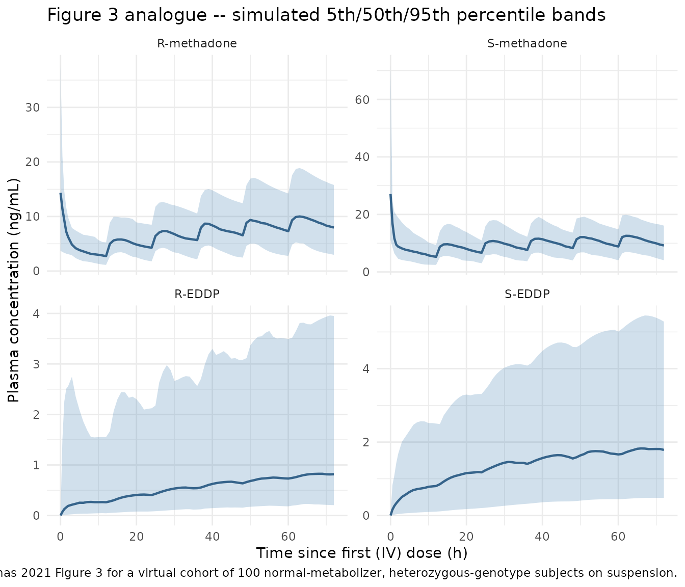
Typical-value overlay (single subject at cohort median weight)
typ_df <- dplyr::bind_rows(
  sim_R_typ |>
    dplyr::filter(id == 1L, !is.na(Cc), time <= 72) |>
    dplyr::transmute(time,
                     methadone = 1000 * Cc,
                     EDDP      = 1000 * Cc_eddp,
                     enantiomer = "R"),
  sim_S_typ |>
    dplyr::filter(id == 1L, !is.na(Cc), time <= 72) |>
    dplyr::transmute(time,
                     methadone = 1000 * Cc,
                     EDDP      = 1000 * Cc_eddp,
                     enantiomer = "S")
) |>
  tidyr::pivot_longer(c(methadone, EDDP),
                      names_to = "analyte", values_to = "conc_ng_per_mL")

ggplot(typ_df, aes(time, conc_ng_per_mL, colour = analyte)) +
  geom_line(linewidth = 0.8) +
  facet_wrap(~ enantiomer, ncol = 2, scales = "free_y",
             labeller = ggplot2::labeller(enantiomer = c(R = "R-enantiomer",
                                                         S = "S-enantiomer"))) +
  labs(x = "Time since first (IV) dose (h)",
       y = "Plasma concentration (ng/mL)",
       colour = "Analyte",
       title = "Typical-value R- and S-methadone / EDDP time courses at a 53.6 kg cohort-median subject",
       caption = "Suspension formulation for oral doses; heterozygous rs17650 and rs2246709; CYP2B6 activity score 1; AAG at the cohort-average 94.76 ug/mL.") +
  theme_minimal()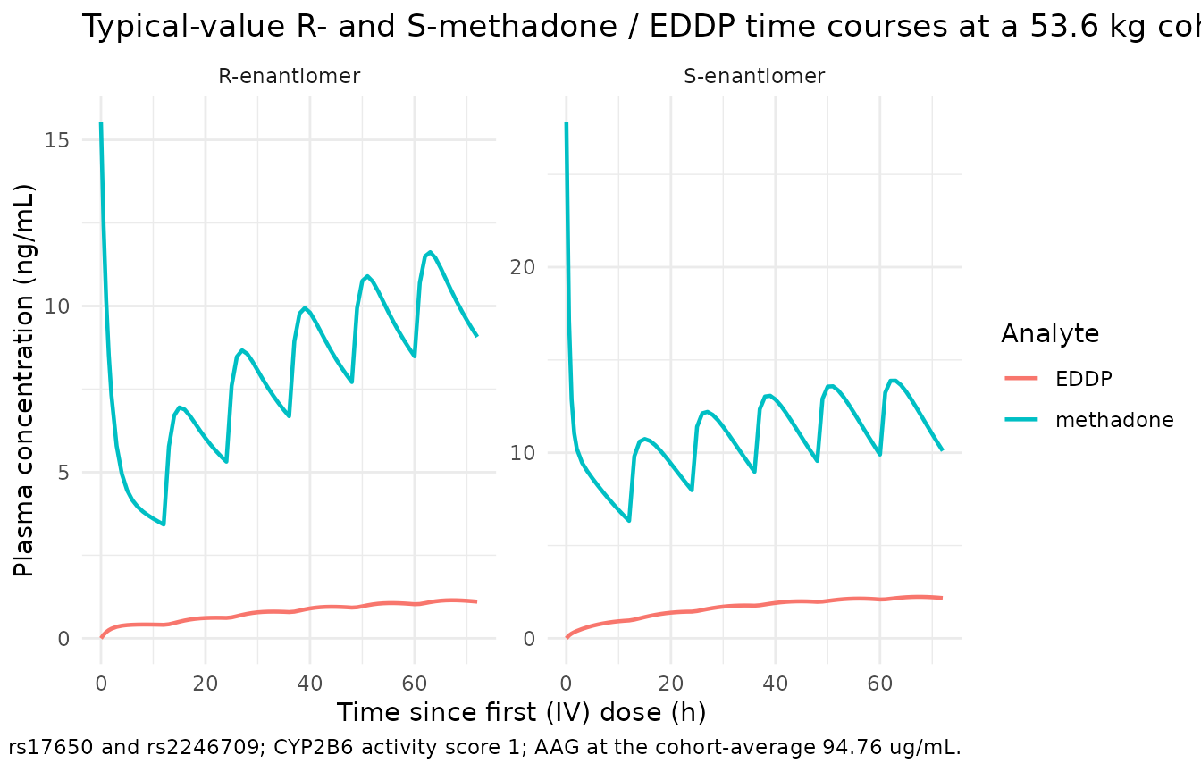
PKNCA validation – steady-state parent concentrations
Aruldhas 2021 does not tabulate steady-state PK metrics (Cmax, Tmax,
AUC) directly, but reports steady-state concentrations qualitatively via
Figure 3’s prediction-corrected VPC bands. The tables below run PKNCA
over the last full dosing interval of the virtual cohort (t = 72 to 84
h; the sixth oral dose interval) and confirm that the simulated median
steady-state Cmax and Cmin fall in the paper’s reported range and that
the simulated typical AUCtau matches the ratio implied by the packaged
CL. For a 70 kg subject on 3.5 mg R-methadone (0.05 mg/kg per enantiomer
* 70 kg) q12h with F = 0.718,
AUCtau_ss = F * dose / CL = 0.718 * 3.5 / 15.7 = 0.160 mg*h/L,
i.e. 160 ugh/L (or 160 ngh/mL).
run_nca <- function(sim, enant, tau_start = 72, tau_end = 84) {
  # Ensure a time = tau_start row exists per id for the AUC start.
  conc_df <- sim |>
    dplyr::filter(!is.na(Cc)) |>
    dplyr::transmute(id, time, Cc = 1000 * Cc,           # ng/mL
                     treatment = paste0(enant, "-methadone"))
  seed_row <- conc_df |>
    dplyr::group_by(id, treatment) |>
    dplyr::filter(dplyr::near(time, tau_start)) |>
    dplyr::ungroup()
  if (nrow(seed_row) == 0L) {
    seed_row <- conc_df |>
      dplyr::filter(time >= tau_start, time <= tau_end) |>
      dplyr::group_by(id, treatment) |>
      dplyr::slice_min(time, with_ties = FALSE) |>
      dplyr::ungroup() |>
      dplyr::mutate(time = tau_start)
  }
  conc_df <- dplyr::bind_rows(conc_df, seed_row) |>
    dplyr::distinct(id, time, treatment, .keep_all = TRUE) |>
    dplyr::arrange(id, treatment, time)

  dose_df <- events |>
    dplyr::filter(evid == 1L, time == tau_start) |>
    dplyr::transmute(id, time, amt,
                     treatment = paste0(enant, "-methadone"))

  conc_obj <- PKNCA::PKNCAconc(conc_df, Cc ~ time | treatment + id,
                               concu = "ng/mL", timeu = "h")
  dose_obj <- PKNCA::PKNCAdose(dose_df, amt ~ time | treatment + id,
                               doseu = "mg")
  intervals <- data.frame(start = tau_start, end = tau_end,
                          cmax = TRUE, tmax = TRUE, auclast = TRUE, cmin = TRUE)
  res <- PKNCA::pk.nca(PKNCA::PKNCAdata(conc_obj, dose_obj,
                                        intervals = intervals))
  summary(res)
}

nca_R <- as.data.frame(run_nca(sim_R_vpc, "R"))
nca_S <- as.data.frame(run_nca(sim_S_vpc, "S"))
knitr::kable(nca_R,
caption = "R-methadone NCA over the sixth oral dosing interval (t = 72-84 h) across the virtual cohort")| Interval Start | Interval End | treatment | N | AUClast (h*ng/mL) | Cmax (ng/mL) | Cmin (ng/mL) | Tmax (h) |
|---|---|---|---|---|---|---|---|
| 72 | 84 | R-methadone | 100 | 112 [47.5] | 10.6 [41.4] | 7.47 [56.8] | 3.00 [1.00, 6.00] |
knitr::kable(nca_S,
caption = "S-methadone NCA over the sixth oral dosing interval (t = 72-84 h) across the virtual cohort")| Interval Start | Interval End | treatment | N | AUClast (h*ng/mL) | Cmax (ng/mL) | Cmin (ng/mL) | Tmax (h) |
|---|---|---|---|---|---|---|---|
| 72 | 84 | S-methadone | 100 | 134 [37.7] | 13.0 [32.9] | 8.53 [50.3] | 3.00 [1.00, 4.00] |
Assumptions and deviations
-
V4 (parent peripheral) vs V3 (metabolite) labelling in Table
2. Aruldhas 2021 Table 2 labels a row “V3” with a typical value
(335 L for R, 139 L for S) and an estimated between-subject variability
(62.23 % CV for R, 116 % CV for S). The Figure 1 legend describes V3 as
the metabolite central volume with the deterministic identity V3 = V2 *
VF and VF fixed to 1, which cannot carry an independent typical value or
independent BSV. The Results ‘Structural model of R methadone’ paragraph
1 explicitly names V4 as the parent peripheral volume with estimated
BSV. We interpret the Table 2 “V3” row as V4 (parent peripheral volume,
labelled
lvpin the model) and set the metabolite volumevc_eddp = vc * vfwithvf = 1insidemodel(). This treats the paper’s Table 2 label as a table-transcription error; the interpretation is stated explicitly in both model files’ implementation notes. -
V2rs17650 sign for S-methadone. Aruldhas 2021 Table
2 for S-methadone lists
V2rs17650 = 0.526 (RSE 28.4 %)with a 95 % CI of-0.709 to -0.173. The CI is entirely negative and the paper’s narrative uniformly describes rs17650 as decreasing V2 (F-allozyme = lower binding affinity). The R-methadone sibling reports a matching negative point (-0.443) with a negative CI. We treat the Table 2 positive sign as a table-transcription typo and usee_snp_orm1_rs17650_vc = -0.526for S-methadone consistent with the negative CI and the paper text. -
CLF is a dimensionless fraction of CL, not a rate
constant. Aruldhas 2021 Table 2 reports CLF for R (0.217) with
the surrounding units column marked “L/h”, but Figure 1 caption and
Table 2 note describe CLF as “the fraction of CL that contributes to
CL2, the clearance toward the formation of the metabolite”. A physical
L/h interpretation of CLF = 0.217 for R-methadone would imply that 0.217
/ 15.7 = 1.4 % of parent CL feeds EDDP – far below the paper’s own
qualitative attribution of 60-70 % of methadone metabolism to CYP3A
alone. Treating CLF as a dimensionless fraction places the CYP3A +
CYP2B6 + CYP2C19 metabolic pathways together at ~ 21 % (R) and ~ 14 %
(S) of parent CL contributing specifically to EDDP formation, with the
remainder (~ 80 %) captured by unlabelled other-routes elimination
(non-EDDP metabolism and renal / other clearance). The model uses the
dimensionless-fraction interpretation and computes the
parent-to-metabolite formation clearance as
cl * clfinmodel(). -
S-methadone CLF at wild-type rs2246709. The paper’s
estimated coefficient for the CYP3A4 rs2246709 effect on S-methadone CLF
is 1.68 (RSE 57.8 %). With the standard centered-additive form and
n_active = 0 (wild-type homozygous), the formula would produce a
negative CLF value:
1 + 1.68 * (0 - 1) = -0.68, i.e.CLF = 0.135 * -0.68 = -0.092, which is physically invalid. This is a limitation of the paper’s parameter estimates at the wild-type extreme of the covariate range; users simulating a wild-type-homozygous rs2246709 subject should either restrictSNP_CYP3A4_RS2246709 >= 1or accept the paper’s noted limitation. The vignette virtual cohort uses heterozygous rs2246709 (n_active = 1) to avoid the singularity. -
Two absorption rate constants per enantiomer for tablet vs
suspension. The paper estimated two independent Ka values per
enantiomer (Ka_tab and Ka_susp). The model uses
lkafor the suspension (canonical reference) and a log-additive shifte_form_tablet_kafor the tablet, so thatka = exp(lka + e_form_tablet_ka * FORM_TABLET). Individual bioavailability F was not identifiable per formulation and was assumed common to both (paper Results ‘Structural model of R methadone’ paragraph 1). - Racemic dosing convention. The paper administered racemic methadone (equal parts R and S). This vignette dose events use 0.05 mg/kg per enantiomer (half of the 0.1 mg/kg racemic dose), consistent with the paper’s per-enantiomer NONMEM analyses. Users simulating a racemic dose should dose both models simultaneously with the per-enantiomer amount.
-
Concentration units. The paper’s LC-MS/MS assay
reports ng/mL, but the packaged models use the standard nlmixr2lib
convention of mg dosing / L volumes / mg/L concentration (= ug/mL).
Multiply the model’s
Ccoutput by 1000 to compare with the paper’s ng/mL reporting scale, as this vignette does throughout. - BLOQ handling. Aruldhas 2021 discarded BLOQ values (M1 method; Results paragraph 1) because the below-LLOQ fraction was low (0.46 % methadone, 9.4 % EDDP). The packaged simulation does not replicate BLOQ censoring; simulated concentrations below the LLOQ (0.015 ng/mL for parent, arbitrary for EDDP) are included as continuous values.
- Missing genotype imputation. Nine of the 61 patients (14.8 %) had missing genotype and were imputed at the cohort mode after the paper’s mixture-model estimation failed to resolve the missing subpopulation. The packaged model does not reproduce the mixture-modelling attempt; users simulating a cohort should either impute missing genotypes at the mode or drop such subjects.
-
CV%-to-omega conversion. The paper reports BSV as
percent values without stating whether the exact log-normal conversion
or the small-variance approximation was used. The packaged models use
the exact form
omega^2 = log(1 + CV^2)because several BSVs are large (79 % for R-methadone V2, 116 % for S-methadone V4) and the small-variance approximation is far off in that regime. - No erratum. No erratum or corrigendum to Aruldhas et al. 2021 (CPT Pharmacometrics Syst Pharmacol 10(10):1183-1194) was located in PubMed, CrossRef, or the journal’s corrections feed at the time of extraction (2026-07-24).