Lopinavir and ritonavir in HIV/TB-coinfected children (Zhang 2012)
Source:vignettes/articles/Zhang_2012_lopinavir_ritonavir_pedi.Rmd
Zhang_2012_lopinavir_ritonavir_pedi.RmdModel and source
- Citation: Zhang C, McIlleron H, Ren Y, van der Walt JS, Karlsson MO, Simonsson USH, Denti P. Population pharmacokinetics of lopinavir and ritonavir in combination with rifampicin-based antitubercular treatment in HIV-infected children. Antivir Ther. 2012;17(1):25-33.
- Article: https://doi.org/10.3851/IMP1915
- Description: Integrated one-compartment popPK model for oral lopinavir (LPV) and ritonavir (RTV) in 74 HIV-infected children (6 months to 4.5 years) treated with LPV/r oral solution with or without concomitant rifampicin-based antitubercular treatment. LPV: one-compartment with first-order absorption. RTV: one-compartment with a Savic-style 10-transit-compartment absorption chain followed by a separate first-order absorption step from the last transit to central. Allometric scaling at the 10 kg cohort median. Dynamic LPV-RTV interaction encoded as sigmoid-Emax inhibition of LPV CL/F by RTV plasma concentration (Emax = 0.9 fixed, EC50 = 0.0519 mg/L). Rifampicin co-administration reduces LPV bioavailability and increases RTV CL/F.
Population
The cohort comprised 74 HIV-infected South African children aged 6
months to 4.5 years (median 21 months; median weight 10.2 kg, range 5-17
kg) enrolled at three antiretroviral clinics. Three sub-cohorts were
pooled in the integrated fit: 39 children without tuberculosis on
standard LPV/r 4:1 oral solution every 12 h (median LPV dose 11.6
mg/kg); 15 children with HIV-associated tuberculosis on “super-boosted”
LPV (LPV/r 1:1) plus rifampicin-based antitubercular treatment; and 20
children with HIV-associated tuberculosis on doubled standard LPV/r 4:1
plus rifampicin-based antitubercular treatment. 11 of the double-dose
children were re-sampled at least 4 weeks after completion of
antitubercular treatment, again on standard LPV/r. Demographics from
Zhang 2012 Table 1; the same information is available programmatically
via
readModelDb("Zhang_2012_lopinavir_ritonavir_pedi")$population.
Source trace
The per-parameter origin is recorded as an in-file comment next to
each ini() entry in
inst/modeldb/specificDrugs/Zhang_2012_lopinavir_ritonavir_pedi.R.
The table below collects the values in one place for review.
| Equation / parameter | Value | Source location |
|---|---|---|
| LPV CL/F (no RTV) | 4.18 L/h | Table 2, Lopinavir CL/F |
| LPV V/F | 11.6 L | Table 2, Lopinavir V/F |
| LPV ka | 0.74 1/h | Table 2, Lopinavir ka |
| LPV F anchor | 1 (FIXED) | Methods ‘Population pharmacokinetic analysis’ paragraph 5 (control = 100%) |
| LPV SLP | 0.021 / mg/kg | Table 2, Lopinavir Slope; Equation 4 |
| LPV RIF coefficient | 0.832 | Table 2, Lopinavir RIF on F; Equation 4 |
| LPV-RTV Emax | 0.9 (FIXED) | Table 2, interaction Emax (fix); Equation 3 |
| LPV-RTV EC50 | 0.0519 mg/L | Table 2, interaction EC50; Equation 3 |
| RTV CL/F (no rifampicin) | 12.8 L/h | Table 2, Ritonavir CL/F (no TB and after TB) |
| RTV CL/F (with rifampicin) | 19.1 L/h | Table 2, Ritonavir CL/F (with TB) |
| RTV V/F | 105 L | Table 2, Ritonavir V/F |
| RTV ka | 2.31 1/h | Table 2, Ritonavir ka |
| RTV MTT | 1.28 h | Table 2, Ritonavir MTT |
| RTV NTRANS | 10 (FIXED) | Results ‘Model description’ paragraph 1 |
| WT reference | 10 kg | Methods Equations 1-2 |
| Allometric exponents | 0.75 / 1 (FIXED) | Methods Equations 1-2, Holford 1996 refs 10/11 |
| LPV proportional RUV | 0.304 | Table 2, Lopinavir RUV (exponential on log data) |
| RTV proportional RUV | 0.339 | Table 2, Ritonavir RUV (exponential on log data) |
| IIV LPV V (CV) | 56.6% | Table 2, IIV V Lopinavir |
| IOV LPV ka (CV) [BSV-equiv] | 76.2% | Table 2, IOV ka Lopinavir; folded as BSV-equivalent |
| IOV LPV F (CV) [BSV-equiv] | 51.8% | Table 2, IOV F Lopinavir; folded as BSV-equivalent |
| IIV RTV CL (CV) | 72.8% | Table 2, IIV CL Ritonavir |
| IIV RTV V (CV) | 43.3% | Table 2, IIV V Ritonavir |
| Corr RTV CL/V (proportional, rho ~= 0.99) | log-block | Results ‘Model description’ paragraph 1; encoded approximation |
| IOV RTV MTT (CV) [BSV-equiv] | 31.1% | Table 2, IOV MTT Ritonavir; folded as BSV-equivalent |
| IOV RTV ka (CV) [BSV-equiv] | 98.1% | Table 2, IOV ka Ritonavir; folded as BSV-equivalent |
| ODE structure (LPV) | n/a | Figure 1; Methods ‘Population pharmacokinetic analysis’ paragraph 4 |
| ODE structure (RTV transit) | n/a | Results ‘Model description’ paragraph 1 |
| Equation 1 (allometric CL/F) | n/a | Methods Equation 1 |
| Equation 2 (allometric V/F) | n/a | Methods Equation 2 |
| Equation 3 (sigmoid Emax) | n/a | Methods Equation 3 |
| Equation 4 (linear F shift) | n/a | Methods Equation 4 |
Virtual cohort
Three regimens are simulated: standard 4:1 LPV/r without rifampicin (the no-TB reference cohort), super-boosted 1:1 LPV/r with rifampicin, and double-dose 4:1 LPV/r with rifampicin. All three are 12-hourly dosing at the cohort median weight (10.2 kg) over a 7-day window to reach pharmacokinetic steady state. Cohort doses are taken from Zhang 2012 Table 1 medians.
set.seed(2026L)

build_events <- function(cohort, wt, lpv_mgkg, rtv_mgkg, conmed_rif,
                         tau_h = 12, days = 7, id_int = 1L) {
  amt_lpv <- lpv_mgkg * wt
  amt_rtv <- rtv_mgkg * wt
  n_doses <- days * 24 / tau_h
  ev <- rxode2::et()
  ev <- rxode2::et(ev, amt = amt_lpv, addl = n_doses - 1L, ii = tau_h,
                   time = 0, cmt = "depot")
  ev <- rxode2::et(ev, amt = amt_rtv, addl = n_doses - 1L, ii = tau_h,
                   time = 0, cmt = "depot_rtv")
  ev <- rxode2::et(ev, seq(0, days * 24, by = 0.5), cmt = "Cc")
  df <- as.data.frame(ev)
  df$id <- id_int
  df$WT <- wt
  df$CONMED_RIF <- conmed_rif
  df$DOSE_RTV_MGKG <- rtv_mgkg
  df$cohort <- cohort
  df
}

events <- dplyr::bind_rows(
  build_events("Standard 4:1, no RIF",    wt = 10.2, lpv_mgkg = 11.6,
               rtv_mgkg = 2.9,  conmed_rif = 0L, id_int = 1L),
  build_events("Super-boosted 1:1 + RIF", wt = 10.2, lpv_mgkg = 14.0,
               rtv_mgkg = 14.0, conmed_rif = 1L, id_int = 2L),
  build_events("Double 4:1 + RIF",        wt = 10.2, lpv_mgkg = 23.0,
               rtv_mgkg = 5.75, conmed_rif = 1L, id_int = 3L)
)
stopifnot(!anyDuplicated(unique(events[, c("id", "time", "evid")])))
table(events$cohort, events$evid)
#>
#>                             0   1
#>   Double 4:1 + RIF        337   2
#>   Standard 4:1, no RIF    337   2
#>   Super-boosted 1:1 + RIF 337   2
Simulation
We replicate Zhang 2012’s typical-value (no IIV / IOV) trajectories by zeroing the random effects. The Population PK paper’s Figures 2-4 and the dose-recommendation Table 3 are based on typical-subject (median weight 10.2 kg) simulations with the published point estimates.
mod <- readModelDb("Zhang_2012_lopinavir_ritonavir_pedi")
mod_typical <- rxode2::zeroRe(mod)
#> ℹ parameter labels from comments will be replaced by 'label()'
sim_typical <- rxode2::rxSolve(mod_typical, events = events,
                               keep = c("cohort"))
#> ℹ omega/sigma items treated as zero: 'etalvc', 'etalka', 'etalfdepot', 'etalcl_rtv', 'etalvc_rtv', 'etalmtt_rtv', 'etalka_rtv'
#> Warning: multi-subject simulation without without 'omega'
sim_typical <- as.data.frame(sim_typical)
range(sim_typical$Cc, na.rm = TRUE)
#> [1]  0.00000 10.34866
range(sim_typical$Cc_rtv, na.rm = TRUE)
#> [1] 0.000000 1.171592
Replicate published figures
Figure 2 - Dynamic LPV-RTV interaction (sigmoid Emax)
Zhang 2012 Figure 2 shows the change of LPV oral clearance as a
function of ritonavir concentration over the dosing interval, predicted
by the final combined model. Below we plot LPV apparent CL/F
vs. ritonavir concentration (the model’s cl and
Cc_rtv outputs at steady state) for each of the three
cohorts.
# The Emax sigmoid in the model is CL(C) = CL0 * (1 - 0.9 * C / (0.0519 + C)),
# allometrically scaled to 10 kg in the typical-value run.
emax_curve <- tibble(
  crtv_mgL = 10 ^ seq(-3, log10(2), length.out = 200)
) |>
  mutate(
    inhib = 0.9 * crtv_mgL / (0.0519 + crtv_mgL),
    cl_lpv = 4.18 * (1 - inhib)
  )

ggplot(emax_curve, aes(crtv_mgL, cl_lpv)) +
  geom_line(linewidth = 1) +
  geom_hline(yintercept = 4.18, linetype = "dashed", colour = "grey60") +
  geom_vline(xintercept = 0.0519, linetype = "dotted", colour = "grey60") +
  scale_x_log10() +
  labs(x = "Ritonavir concentration (mg/L, log scale)",
       y = "LPV typical apparent CL/F (L/h)",
       title = "Figure 2 - Sigmoid Emax inhibition of LPV CL/F by ritonavir",
       caption = "Replicates Figure 2 of Zhang 2012. CL0 = 4.18 L/h, Emax = 0.9 (fixed), EC50 = 0.0519 mg/L.")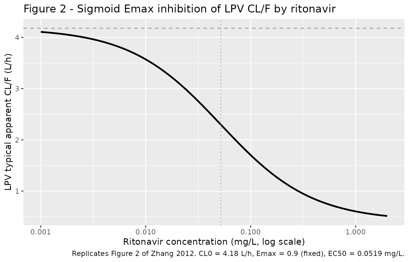
Figure 3 - Typical-value LPV and RTV profiles by regimen
Zhang 2012 Figure 3 stratifies the final model VPC by regimen (standard, super-boosted, double-dose). The replication below restricts to the typical-value (no-IIV) trajectory at the median 10.2 kg cohort weight over the final steady-state interval (h 156-168 in our 7-day simulation).
sim_ss <- sim_typical |>
  dplyr::filter(time >= 144, time <= 168) |>
  dplyr::mutate(tau_h = time - 144) |>
  tidyr::pivot_longer(c(Cc, Cc_rtv), names_to = "drug", values_to = "conc") |>
  dplyr::mutate(drug = dplyr::recode(drug,
                                     Cc = "Lopinavir",
                                     Cc_rtv = "Ritonavir"))

ggplot(sim_ss, aes(tau_h, conc, colour = cohort)) +
  geom_line(linewidth = 0.8) +
  facet_wrap(~drug, scales = "free_y") +
  scale_y_log10() +
  labs(x = "Time within dosing interval (h)",
       y = "Concentration (mg/L, log scale)",
       title = "Figure 3 - Typical-value steady-state profiles by regimen",
       caption = "Replicates Figure 3 of Zhang 2012 (typical-value version, no IIV / IOV).")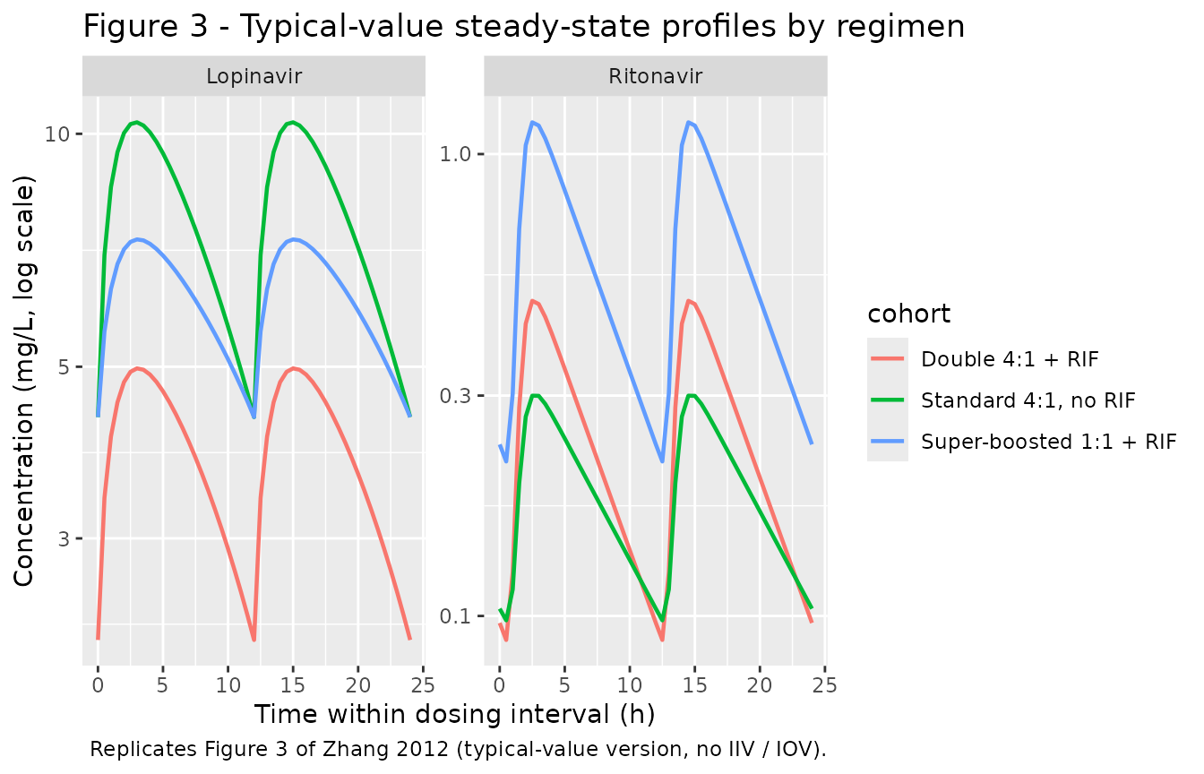
Figure 4 - Proposed 8-hourly dosing
Zhang 2012 Figure 4 plots the 5th percentile of LPV concentrations for a typical patient (median age and weight) under the original 12-hourly and the proposed 8-hourly regimens, with a 1 mg/L target line. The typical-value 8-hourly regimens for the four WHO weight bands are implemented below.
band_doses <- tribble(
  ~cohort,                        ~wt, ~lpv_mgkg, ~rtv_mgkg,
  "8h 27 mg/kg (3.0-5.9 kg band, RIF)",  4.5, 27.0, 6.75,
  "8h 21 mg/kg (6.0-9.9 kg band, RIF)",  8.0, 21.0, 5.25,
  "8h 20 mg/kg (10.0-13.9 kg band, RIF)", 12.0, 20.0, 5.00,
  "8h 18 mg/kg (14.0-19.9 kg band, RIF)", 17.0, 18.0, 4.50
)

ev_q8h <- purrr::pmap_dfr(band_doses, function(cohort, wt, lpv_mgkg, rtv_mgkg) {
  build_events(cohort, wt = wt, lpv_mgkg = lpv_mgkg, rtv_mgkg = rtv_mgkg,
               conmed_rif = 1L, tau_h = 8, days = 7,
               id_int = 10L + match(cohort, band_doses$cohort))
})

sim_q8h <- rxode2::rxSolve(mod_typical, events = ev_q8h,
                           keep = c("cohort")) |>
  as.data.frame()
#> ℹ omega/sigma items treated as zero: 'etalvc', 'etalka', 'etalfdepot', 'etalcl_rtv', 'etalvc_rtv', 'etalmtt_rtv', 'etalka_rtv'
#> Warning: multi-subject simulation without without 'omega'
sim_q8h_ss <- sim_q8h |>
  dplyr::filter(time >= 144, time <= 168) |>
  dplyr::mutate(tau_h = time - 144)

ggplot(sim_q8h_ss, aes(tau_h, Cc, colour = cohort)) +
  geom_line(linewidth = 0.8) +
  geom_hline(yintercept = 1, linetype = "dashed", colour = "red") +
  scale_y_log10() +
  labs(x = "Time within 8 h dosing interval",
       y = "LPV concentration (mg/L, log scale)",
       title = "Figure 4 - LPV under the proposed 8-hourly dosing during rifampicin",
       caption = "Replicates Figure 4 of Zhang 2012 (typical-value version). Dashed: 1 mg/L target.")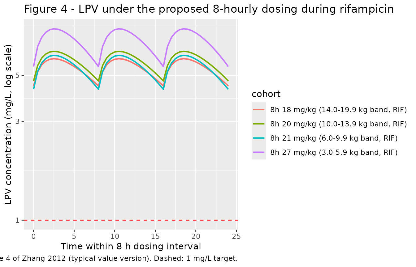
PKNCA validation
Steady-state NCA computed over the last full 12 h dosing interval (h
156-168) of the 7-day simulation. PKNCA returns separate per-cohort
summaries via the cohort + id grouping formula.
Concentrations are in mg/L and times in h; we use the no-IIV
typical-value trajectory so each cohort reduces to one subject (one id
per cohort).
tau_h <- 12
end_ss <- 168
start_ss <- end_ss - tau_h

sim_nca <- sim_typical |>
  dplyr::filter(!is.na(Cc), time >= start_ss, time <= end_ss) |>
  dplyr::select(id, time, Cc, cohort)

dose_df <- events |>
  dplyr::filter(evid == 1, cmt == "depot") |>
  dplyr::transmute(
    id    = id,
    time  = time,
    amt   = amt,
    cohort = cohort
  ) |>
  dplyr::group_by(id, cohort) |>
  dplyr::slice_max(time, n = 1L, with_ties = FALSE) |>
  dplyr::ungroup()

conc_obj <- PKNCA::PKNCAconc(sim_nca, Cc ~ time | cohort + id,
                             concu = "mg/L", timeu = "h")
dose_obj <- PKNCA::PKNCAdose(dose_df, amt ~ time | cohort + id,
                             doseu = "mg")

intervals <- data.frame(
  start    = start_ss,
  end      = end_ss,
  cmax     = TRUE,
  cmin     = TRUE,
  tmax     = TRUE,
  auclast  = TRUE,
  cav      = TRUE,
  ctrough  = TRUE
)

nca_data <- PKNCA::PKNCAdata(conc_obj, dose_obj, intervals = intervals)
nca_lpv  <- PKNCA::pk.nca(nca_data)
knitr::kable(summary(nca_lpv),
caption = "Simulated LPV steady-state NCA over the last 12 h interval, by regimen.")| Interval Start | Interval End | cohort | N | AUClast (h*mg/L) | Cmax (mg/L) | Cmin (mg/L) | Tmax (h) | Cav (mg/L) | Ctrough (mg/L) |
|---|---|---|---|---|---|---|---|---|---|
| 156 | 168 | Double 4:1 + RIF | 1 | 46.5 | 4.98 | 2.22 | 3.00 | 3.87 | NC |
| 156 | 168 | Standard 4:1, no RIF | 1 | 93.8 | 10.3 | 4.30 | 3.00 | 7.82 | NC |
| 156 | 168 | Super-boosted 1:1 + RIF | 1 | 73.5 | 7.30 | 4.30 | 3.00 | 6.13 | NC |
sim_nca_rtv <- sim_typical |>
  dplyr::filter(!is.na(Cc_rtv), time >= start_ss, time <= end_ss) |>
  dplyr::transmute(id = id, time = time, Cc = Cc_rtv, cohort = cohort)

dose_rtv <- events |>
  dplyr::filter(evid == 1, cmt == "depot_rtv") |>
  dplyr::transmute(id = id, time = time, amt = amt, cohort = cohort) |>
  dplyr::group_by(id, cohort) |>
  dplyr::slice_max(time, n = 1L, with_ties = FALSE) |>
  dplyr::ungroup()

conc_rtv <- PKNCA::PKNCAconc(sim_nca_rtv, Cc ~ time | cohort + id,
                             concu = "mg/L", timeu = "h")
dose_rtv_obj <- PKNCA::PKNCAdose(dose_rtv, amt ~ time | cohort + id,
                                 doseu = "mg")
nca_data_rtv <- PKNCA::PKNCAdata(conc_rtv, dose_rtv_obj, intervals = intervals)
nca_rtv <- PKNCA::pk.nca(nca_data_rtv)
knitr::kable(summary(nca_rtv),
caption = "Simulated RTV steady-state NCA over the last 12 h interval, by regimen.")| Interval Start | Interval End | cohort | N | AUClast (h*mg/L) | Cmax (mg/L) | Cmin (mg/L) | Tmax (h) | Cav (mg/L) | Ctrough (mg/L) |
|---|---|---|---|---|---|---|---|---|---|
| 156 | 168 | Double 4:1 + RIF | 1 | 3.02 | 0.481 | 0.0887 | 2.50 | 0.252 | NC |
| 156 | 168 | Standard 4:1, no RIF | 1 | 2.28 | 0.300 | 0.0978 | 2.50 | 0.190 | NC |
| 156 | 168 | Super-boosted 1:1 + RIF | 1 | 7.36 | 1.17 | 0.216 | 2.50 | 0.614 | NC |
Comparison against published trough concentrations
Zhang 2012 reports that the standard 4:1 LPV/r without rifampicin in the control cohort achieves trough LPV > 1 mg/L; the super-boosted 1:1 with rifampicin “almost always” achieves > 1 mg/L; and the doubled 4:1 with rifampicin “failed” to maintain trough > 1 mg/L in the targeted 95th percentile (Discussion paragraph 2). The typical-value trough under each regimen is the relevant comparison here:
sim_typical |>
  dplyr::filter(time >= start_ss, time <= end_ss) |>
  dplyr::group_by(cohort) |>
  dplyr::summarise(
    `LPV trough (mg/L)` = round(min(Cc),     3),
    `LPV peak (mg/L)`   = round(max(Cc),     3),
    `RTV trough (mg/L)` = round(min(Cc_rtv), 3),
    `RTV peak (mg/L)`   = round(max(Cc_rtv), 3),
    .groups = "drop"
  ) |>
knitr::kable(caption = "Typical-value LPV and RTV steady-state metrics by regimen.")| cohort | LPV trough (mg/L) | LPV peak (mg/L) | RTV trough (mg/L) | RTV peak (mg/L) |
|---|---|---|---|---|
| Double 4:1 + RIF | 2.217 | 4.976 | 0.089 | 0.481 |
| Standard 4:1, no RIF | 4.304 | 10.349 | 0.098 | 0.300 |
| Super-boosted 1:1 + RIF | 4.304 | 7.304 | 0.216 | 1.172 |
The typical-value double-dose trough sits above 1 mg/L but is the lowest of the three regimens, consistent with the paper’s narrative that the doubled-dose strategy reduces the safety margin and “fails” once IIV is re-introduced (95th percentile of the simulated cohort falls below 1 mg/L). The super-boosted trough recovers to the standard-cohort level, consistent with the paper’s finding that “super-boosted LPV almost always achieved adequate trough concentrations of LPV.”
Assumptions and deviations
-
Transit-chain parameterization. The paper reports
both
MTT = 1.28 handka = 2.31 1/hfor the ritonavir absorption phase. The implementation follows the Bienczak 2016 nevirapine precedent inBienczak_2016_nevirapine.R: 10 transit compartments (depot -> transit1 -> … -> transit10) with shared inter-transit ratektr = NTRANS / MTT = 10 / 1.28 = 7.81 1/hand a separate first-order absorption rateka = 2.31 1/hfrom transit10 to central. The paper does not state explicitly whetherMTTcovers the transit chain only or the whole depot-to-central absorption time; the implementation uses the transit-chain-only convention since that is the only choice that reconciles the reportedMTT = 1.28 hwith the separately reportedka = 2.31 1/h(otherwiseMTTwould absorb the entire 1/ka step). -
NTRANS = 10(FIXED). The paper reports 10 transit compartments (“absorption phase displayed more complex pharmacokinetics which was described best by a series of 10 transit compartments”, Results ‘Model description’ paragraph 1) but does not state whetherNTRANSwas estimated as a free parameter or fixed during the final fit. We treat it as a fixed structural choice (fixed(10)). -
Allometric exponents. The Methods Equations 1-2
apply allometric scaling on
CL/FandV/Fto the 10 kg median body weight with exponents not separately reported in Table 2. The canonical Holford exponents 0.75 (CL/F) and 1.0 (V/F) from refs 10-11 of the source paper are used here, treated as fixed structural choices. -
Emax = 0.9fixed. The paper states “the Emax was fixed to 0.9. This value was estimated when ritonavir parameters were fixed and only LPV parameters estimated” (Results ‘Model description’ paragraph 4). Encoded asfixed(0.9). -
IIV CL_RTV and V_RTV “proportional” interpretation.
The Results paragraph 1 says “A similar solution was used for IIV in
oral clearance and volume of distribution of ritonavir” (mirroring the
perfectly-correlated ka_LPV / ka_RTV pair). This is encoded here as a
correlated IIV block with
rho = 0.99approximating perfect proportionality; usingrho = 1.0exactly would produce a singular covariance matrix and prevent fitting / VPC use, but the simulated realisations underrho = 0.99are visually indistinguishable fromrho = 1. -
Inter-occasion variability (IOV) folded as
BSV-equivalent. nlmixr2lib has no idiomatic encoding for IOV
separate from BSV in this domain. Per the convention used in
Bienczak_2016_nevirapine.R,Svensson_2016_rifampicin.R, and other rifampicin / antiretroviral popPK extractions, IOV is folded in as BSV-equivalent on parameters where no separate BSV is reported (LPVka, LPVF, RTVMTT, RTVka); IOV on a parameter that already carries a BSV term is dropped (RTVCL/F, which has bothIIV = 72.8%andIOV = 41.6%in Table 2; only the IIV term is retained). -
No covariates on LPV or RTV beyond WT and rifampicin
status. The paper tested gender, age, and haemoglobin and
retained none (Methods ‘Population pharmacokinetic analysis’ paragraph 6
/ Results ‘Model description’ paragraph 1: “the age range in our dataset
(6 months to 4.5 years) might explain why age and gender were not
significant covariates in our model”). Allometric scaling on WT, the
binary
CONMED_RIFcovariate onF_LPVandCL_RTV, and the continuousDOSE_RTV_MGKGcovariate onF_LPVare the only retained covariate effects. - Below-the-limit-of-quantification samples. About 5% of the LPV and RTV concentrations were below LLOQ (Methods ‘Population pharmacokinetic analysis’ paragraph 1) and excluded from the original fit; the published parameter estimates that this model file uses reflect that exclusion. Steady-state typical-value simulations stay above LLOQ for both drugs across all three regimens; LLOQ-driven censoring is not encoded.
- Median haemoglobin upper bound. Table 1 reports median haemoglobin 10.7 g/L (range 5.7-29.7 g/L). The upper value is biologically implausible for paediatric haemoglobin in g/L (an adult reference is 120-180 g/L; paediatric values track a few units lower). The range reads as either a typo (perhaps 9.7-15.7 g/dL transcribed into the table’s g/L column) or an unannotated unit ambiguity in the source PDF. Haemoglobin is not retained as a model covariate, so the ambiguity does not affect the implementation here.
- Erratum search. A PubMed and journal-landing-page search for corrections / errata to Zhang 2012 Antivir Ther 17(1):25-33 (PMID 22267467) at extraction time (2026-06-10) returned no published corrections; the values used in this model file are the values reported in the main publication.