Automated NODE-LASSO model development (Braem 2026) • nlmixr2lib

Model and source

Braem 2026 is a methods paper. It proposes an automated pharmacometric model-development workflow in which a low-dimensional neural ODE (NODE) is fitted to the data first, its learned right-hand side is read out as derivative-versus-state data, and LASSO regression then selects an explicit, mechanism-based set of functions that can replace the neural network. The paper demonstrates it on three examples: neonatal weight, simulated bi-exponential PK, and warfarin PK/PD.

Three of those models are packaged here.

model_names <- c(
  "Bram_2026_warfarin_node",
  "Bram_2026_biexponential",
  "Bram_2026_biexponential_2cmt"
)
uis <- lapply(model_names, function(n) rxode2::rxode(readModelDb(n)))
#> ℹ parameter labels from comments will be replaced by 'label()'
names(uis) <- model_names

Citation: Braem DS, Steiert B, Steffens B, Pfister M, Koch G. Automated pharmacometric model development by leveraging low-dimensional neural ODEs and LASSO regression. CPT Pharmacometrics Syst Pharmacol. 2026. doi:10.1002/psp4.70285. Parameter estimates are from the article’s Data S2 code deposit (Monolix project Warf_node_mlx_file_ind, populationParameters.txt); no parameter table appears in the article text. Warfarin data from O’Reilly RA, Aggeler PM. Circulation. 1968;38(1):169-177. doi:10.1161/01.cir.38.1.169.
Article: https://doi.org/10.1002/psp4.70285
Supporting Information (Tables S1/S2, derivations, Figures S1-S3) and the authored Data S2 code deposit are open access alongside the article.

What is packaged, and what is not

Braem 2026 prints no parameter table anywhere in the article text – Table 1 reports only mean absolute relative errors. Every value used here comes from the Supporting Information or from the Data S2 code deposit, and the three models below are exactly those for which estimates exist.

Coverage of Braem 2026 in nlmixr2lib.
Paper model	Packaged	Where the numbers are
Warfarin NODE (Eq 16)	yes – `Bram_2026_warfarin_node`	Data S2, Monolix run `Warf_node_mlx_file_ind/populationParameters.txt`
Bi-exponential proposed one-state model (Eq 20)	yes – `Bram_2026_biexponential`	Table S2 (`k`, `p`) plus an exact inversion for the other two
Bi-exponential reference two-compartment model (Eq 14)	yes – `Bram_2026_biexponential_2cmt`	Table S2 macro-parameters, inverted to micro-constants
Neonatal weight model (Eq 18)	no	`kw, kt, q, p, W0` are stated to have been estimated; values printed nowhere
Warfarin LASSO-proposed model (Eq 24)	no	parameters stated to have been estimated; values printed nowhere
Warfarin reference Imax model (Eq 25)	no	only its BIC (2166) is reported

The two omitted warfarin/weight models are excluded on the initial-versus-final rule, not for want of looking. Figure 4 of the article does carry readable numbers, and the Supporting Information even ships one derivative vector verbatim – but the Figure 4 caption states that the red dashed line is “the through LASSO identified function”, i.e. the step-3 output that becomes the starting values for the step-4 fit. Those are initial estimates, and shipping them as final would misrepresent the paper. This is a general shape worth naming: a derivative-versus-state plot in a NODE-distillation paper is an initial-estimate figure by construction.

Population

The warfarin example uses the warfarin PK/PD dataset distributed as an example with Monolix and nlmixr, originating from O’Reilly and Aggeler (1968): 32 adults given a single oral dose, with a median of 6 (IQR 6-10) plasma warfarin concentrations and 7 (IQR 7-8) prothrombin complex activity (PCA) observations each, over 144 h (Braem 2026 Section 2.3.3). The deposited warfarin_pkpd_data.csv shows doses of 60-153 mg (mean 105 mg). Braem 2026 gives no baseline demographic table, and the deposited file carries no age, weight, sex or race column.

The bi-exponential example is not a real study at all: Braem 2026 Section 2.3.2 simulated 50 subjects from the two-compartment model of Equation 14, with 7 concentration measurements over 24 h, as a sensitivity analysis asking whether the workflow recovers a usable structure for data that arose from a model with a latent state.

str(uis[["Bram_2026_warfarin_node"]]$population)
#> List of 7
#>  $ species      : chr "human"
#>  $ n_subjects   : num 32
#>  $ n_studies    : num 1
#>  $ disease_state: chr "Adults initiating oral anticoagulation; the warfarin PK/PD dataset distributed as an example with Monolix and n"| __truncated__
#>  $ dose_range   : chr "Single oral dose, 60-153 mg (mean 105 mg) per the deposited warfarin_pkpd_data.csv; approximately 1.5 mg/kg."
#>  $ observations : chr "Median 6 (IQR 6-10) warfarin plasma concentrations and 7 (IQR 7-8) prothrombin complex activity observations pe"| __truncated__
#>  $ notes        : chr "Braem 2026 reports no baseline demographic table for this dataset; age, weight, sex and race are not available "| __truncated__

Source trace

Per-parameter origin is recorded as an in-file comment beside each ini() entry. Collected here for review:

Source trace for all three packaged models.
Equation / parameter	Value	Source location
PK structure: 1-cmt oral with lag	n/a	Eq 16, first three lines (Monolix `pkmodel(Tlag, ka, V, Cl)`)
PD structure: indirect response, NN production	n/a	Eq 16, fourth line; expanded in Data S2 `Warf_node_converted.txt`
Softplus activation, beta	20	Supporting Information Eq (2); pmxNODE default
`ltlag`, `lka`, `lvc`, `lcl`	0.8083 h, 1.241 /h, 8.003 L, 0.1308 L/h	Data S2 `Warf_node_mlx_file_ind/populationParameters.txt`
`lrbase`, `lkout`	95.15 %, 0.04075 /h	same file (`R0_pop`, `kout_pop`)
`nn_w1_rc_`, `nn_b1_rc_`, `nn_w2_rc_*`	15 values	same file (`Wrc_1`, `brc_1`, `Wrc_2*`)
21 IIV variances	omega squared	same file (`omega_*`); Monolix reports SD, nlmixr2 takes variance
Residual error, both outputs	`combined1(a, b)`	Data S2 `Warf_node_mlx_file_ind.mlxtran`, DEFINITION block
Proposed one-state model structure	n/a	Eq 20; multiple-dose `tad` form in Supporting Information
`lkel` (paper `k` / `r`), `lkdist` (paper `p`)	0.12 /h, 0.46 /h	Table S2
`lwdist` (paper `w` / `q`), `lvc`	0.1717 /h, 1/10.1	inverted from Table S2 `A'` = 5.1, `B'` = 5.0 (derived below)
Two-compartment reference structure	n/a	Eq 14
`lcl`, `lvc`, `lq`, `lvp`	macro-to-micro inversion	Table S2 A = 5.1, alpha = 0.46, B = 5.0, beta = 0.12 (derived below)

Part 1 – the warfarin neural ODE

The PD production rate of this indirect-response model is a one-hidden-layer, five-neuron softplus network of the plasma concentration:

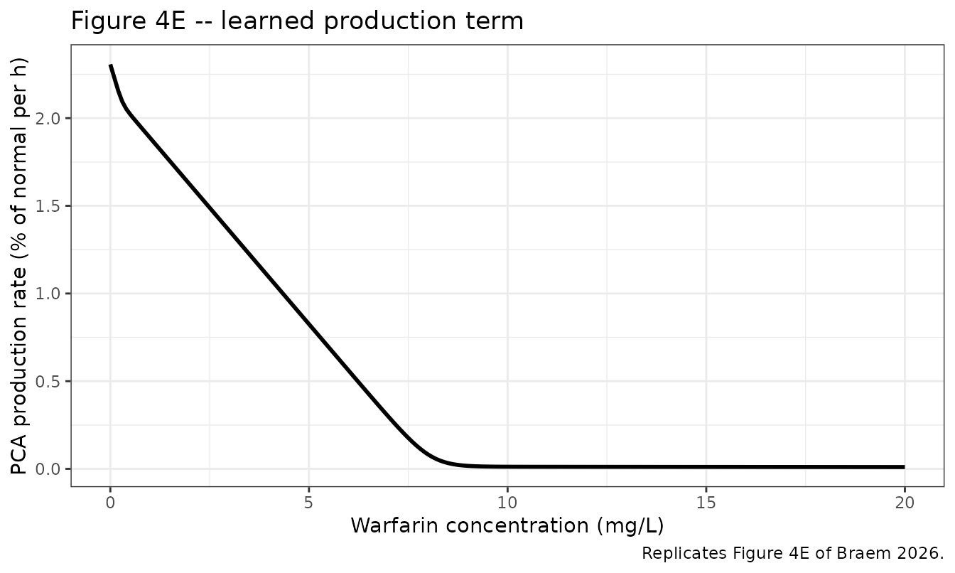
$\frac{dPCA}{dt} = \sum_{j=1}^{5} w^{(2)}_j \cdot \frac{1}{\beta}\log\!\left(1 + e^{\,\beta \left(-\left(w^{(1)}_j\right)^2 C_c\right) + b^{(1)}_j}\right) - k_{out}\, PCA .$

Gate 1 – the network reproduces Figure 4E

Braem 2026 Figure 4E plots this network’s output against concentration, running from about 2.0 at the left-hand edge of the plotted range down to approximately 0 by 15 mg/L. Evaluating the packaged parameters directly is a check on the transcription and on the operator precedence inside the softplus, which the deposited code writes as beta * (-(w^2) * Cc) + b rather than beta * (-(w^2) * Cc + b).

ini_w <- uis[["Bram_2026_warfarin_node"]]$theta
nn_eval <- function(cc) {
  h <- vapply(1:5, function(j) {
    w1 <- ini_w[[paste0("nn_w1_rc_", j)]]
    b1 <- ini_w[[paste0("nn_b1_rc_", j)]]
    log(1 + exp(20 * (-(w1^2) * cc) + b1)) / 20
  }, numeric(1))
  w2 <- vapply(1:5, function(j) ini_w[[paste0("nn_w2_rc_", j)]], numeric(1))
  sum(w2 * h)
}
nn_curve <- tibble(Cc = seq(0, 20, by = 0.1)) |>
  mutate(production = vapply(Cc, nn_eval, numeric(1)))

edge_left  <- nn_eval(0.5)
edge_right <- nn_eval(15)
c(`NN at Cc = 0.5` = edge_left, `NN at Cc = 15` = edge_right)
#> NN at Cc = 0.5  NN at Cc = 15 
#>     2.02183850     0.01102662

# Deterministic evaluation of published constants: a tight bound is correct
# here, there is no cohort and no RNG involved.
stopifnot(
  abs(edge_left - 2.0) < 0.1,   # Figure 4E left-hand edge reads 2.0
  edge_right < 0.1,             # Figure 4E has decayed to ~0 by 15 mg/L
  all(diff(nn_curve$production) <= 0)  # softplus with negated squared weights is monotone
)

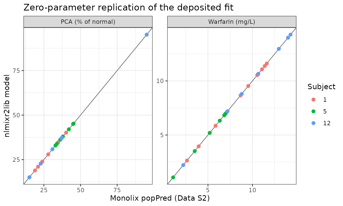
Gate 2 – the packaged model reproduces Monolix’s own population predictions

The Data S2 deposit contains the fitted run’s predictions_ycp.txt and predictions_ypca.txt, which hold Monolix’s population predictions (popPred, i.e. all etas at zero) at every observation time of every subject. Because the population prediction depends on nothing but the subject’s dose, solving the packaged model with zeroRe() at that dose must reproduce them. This is a zero-parameter gate: it simultaneously confirms all 21 estimates, the ODE structure, the softplus precedence, and the PCA(0) = rbase initial condition.

Three subjects spanning the dose range are transcribed below.

published_pred <- tibble::tribble(
  ~id, ~amt, ~time, ~output, ~popPred,
  # --- subject 1, 100 mg (Data S2 predictions_ypca.txt / predictions_ycp.txt)
  1L, 100,  24,   "PCA", 37.0193,
  1L, 100,  36,   "PCA", 23.9270,
  1L, 100,  48,   "PCA", 18.9423,
  1L, 100,  72,   "PCA", 21.0226,
  1L, 100,  96,   "PCA", 27.9879,
  1L, 100, 120,   "PCA", 34.7860,
  1L, 100, 144,   "PCA", 40.1675,
  1L, 100,   1,   "Cc",   2.6408,
  1L, 100,   2,   "Cc",   9.5320,
  1L, 100,   3,   "Cc",  11.3820,
  1L, 100,   6,   "Cc",  11.6114,
  1L, 100,   9,   "Cc",  11.0746,
  1L, 100,  12,   "Cc",  10.5451,
  1L, 100,  24,   "Cc",   8.6672,
  1L, 100,  36,   "Cc",   7.1238,
  1L, 100,  48,   "Cc",   5.8551,
  1L, 100,  72,   "Cc",   3.9554,
  # --- subject 5, 60 mg
  5L,  60,   0,   "PCA", 95.1495,
  5L,  60,  24,   "PCA", 44.9263,
  5L,  60,  36,   "PCA", 36.1485,
  5L,  60,  48,   "PCA", 32.8811,
  5L,  60,  72,   "PCA", 33.8858,
  5L,  60,  96,   "PCA", 37.9848,
  5L,  60, 120,   "PCA", 42.0326,
  5L,  60, 144,   "PCA", 45.2464,
  5L,  60,   3,   "Cc",   6.8292,
  5L,  60,   6,   "Cc",   6.9669,
  5L,  60,  12,   "Cc",   6.3271,
  5L,  60,  24,   "Cc",   5.2003,
  5L,  60,  48,   "Cc",   3.5131,
  5L,  60, 120,   "Cc",   1.0831,
  # --- subject 12, 123 mg
  12L, 123,   0,  "PCA", 95.1495,
  12L, 123,  24,  "PCA", 36.9130,
  12L, 123,  36,  "PCA", 22.7836,
  12L, 123,  48,  "PCA", 15.0629,
  12L, 123,  72,  "PCA", 15.1787,
  12L, 123,  96,  "PCA", 22.8206,
  12L, 123, 120,  "PCA", 30.8389,
  12L, 123, 144,  "PCA", 37.3307,
  12L, 123, 1.5,  "Cc",   8.7979,
  12L, 123,   3,  "Cc",  13.9998,
  12L, 123,   6,  "Cc",  14.2821,
  12L, 123,  12,  "Cc",  12.9705,
  12L, 123,  24,  "Cc",  10.6607,
  12L, 123,  48,  "Cc",   7.2018,
  12L, 123, 120,  "Cc",   2.2203
)

warf_typical <- rxode2::zeroRe(uis[["Bram_2026_warfarin_node"]])

solve_one <- function(subject_id, dose, times) {
  ev <- rxode2::et(amt = dose, cmt = "depot") |>
    rxode2::et(sort(unique(c(0, times))))
  ev <- as.data.frame(ev)
  # Two `~` endpoints: put dvid on every observation row. rxSolve returns
  # BOTH Cc and PCA as columns regardless, so one grid suffices.
  ev$dvid <- ifelse(ev$evid == 0, 1L, NA_integer_)
  s <- rxode2::rxSolve(warf_typical, ev, returnType = "data.frame")
  tibble(id = subject_id, time = s$time, Cc = s$Cc, PCA = s$PCA)
}

simulated_pred <- published_pred |>
  group_by(id) |>
  group_modify(function(d, k) {
    solve_one(k$id, d$amt[1], d$time) |> select(-id)
  }) |>
  ungroup()
#> ℹ omega/sigma items treated as zero: 'etaltlag', 'etalka', 'etalvc', 'etalcl', 'etalrbase', 'etalkout', 'etann_w1_rc_1', 'etann_w1_rc_2', 'etann_w1_rc_3', 'etann_w1_rc_4', 'etann_w1_rc_5', 'etann_b1_rc_1', 'etann_b1_rc_2', 'etann_b1_rc_3', 'etann_b1_rc_4', 'etann_b1_rc_5', 'etann_w2_rc_1', 'etann_w2_rc_2', 'etann_w2_rc_3', 'etann_w2_rc_4', 'etann_w2_rc_5'
#> ℹ omega/sigma items treated as zero: 'etaltlag', 'etalka', 'etalvc', 'etalcl', 'etalrbase', 'etalkout', 'etann_w1_rc_1', 'etann_w1_rc_2', 'etann_w1_rc_3', 'etann_w1_rc_4', 'etann_w1_rc_5', 'etann_b1_rc_1', 'etann_b1_rc_2', 'etann_b1_rc_3', 'etann_b1_rc_4', 'etann_b1_rc_5', 'etann_w2_rc_1', 'etann_w2_rc_2', 'etann_w2_rc_3', 'etann_w2_rc_4', 'etann_w2_rc_5'
#> ℹ omega/sigma items treated as zero: 'etaltlag', 'etalka', 'etalvc', 'etalcl', 'etalrbase', 'etalkout', 'etann_w1_rc_1', 'etann_w1_rc_2', 'etann_w1_rc_3', 'etann_w1_rc_4', 'etann_w1_rc_5', 'etann_b1_rc_1', 'etann_b1_rc_2', 'etann_b1_rc_3', 'etann_b1_rc_4', 'etann_b1_rc_5', 'etann_w2_rc_1', 'etann_w2_rc_2', 'etann_w2_rc_3', 'etann_w2_rc_4', 'etann_w2_rc_5'

poppred_check <- published_pred |>
  left_join(simulated_pred, by = c("id", "time")) |>
  mutate(simulated = if_else(output == "PCA", PCA, Cc),
         pct_diff  = 100 * (simulated - popPred) / popPred) |>
  filter(popPred > 0)   # the pre-absorption Cc rows are exactly 0 in both

max_poppred_diff <- max(abs(poppred_check$pct_diff))
max_poppred_diff
#> [1] 0.2299427

# Deterministic (zeroRe, fixed doses, no RNG): a tight bound is correct.
# Realised 0.213% here; the residual is Monolix's own reporting precision and
# integrator tolerance. A single mis-transcribed weight, bias or rate moves
# this by whole percent or more.
stopifnot(max_poppred_diff < 1)

Packaged model vs Monolix popPred from the Data S2 deposit.
Subject	Output	Observations	max \|% diff\|
1	Cc	10	0.001
1	PCA	7	0.051
5	Cc	6	0.003
5	PCA	8	0.230
12	Cc	7	0.001
12	PCA	8	0.109

The baseline is deliberately not a steady state

Because the network replaces the production term outright, nothing constrains it to balance kout * PCA0 at zero concentration. It does not:

kin_implied  <- nn_eval(0)
loss_at_base <- ini_w[["lkout"]] |> exp() * exp(ini_w[["lrbase"]])
c(`network production at Cc = 0` = kin_implied,
  `kout * PCA0`                  = loss_at_base)
#> network production at Cc = 0                  kout * PCA0 
#>                     2.306617                     3.877141

stopifnot(kin_implied < loss_at_base)   # deterministic; both are fixed constants

So PCA declines from baseline even with no drug present. That asymmetry is precisely what Braem 2026 repairs in the LASSO-distilled model of Equation 24, by rearranging the identified functions and introducing kin = k + q “to ensure steady-state behavior when no drug is given”. It is worth seeing in the packaged NODE, because it is the concrete cost of a black-box right-hand side that the paper’s whole workflow exists to convert into an interpretable one.

Simulated cohort and PKNCA

# rxSetSeed() fixes rxode2's stream per solver thread, not across thread
# counts, so this cohort differs between machines. Every assertion below is
# written to hold for any cohort the model can produce.
rxode2::rxSetSeed(20260903)
n_sub <- 100L   # well under the 200-per-arm cap

obs_times <- c(seq(0, 12, by = 0.5), seq(14, 144, by = 2))
cohort_ev <- rxode2::et(amt = 100, cmt = "depot") |> rxode2::et(obs_times)
cohort_ev <- as.data.frame(cohort_ev)
cohort_ev$dvid <- ifelse(cohort_ev$evid == 0, 1L, NA_integer_)
cohort_ev$treatment <- "100 mg single oral dose"

sim <- rxode2::rxSolve(uis[["Bram_2026_warfarin_node"]], cohort_ev,
                       nSub = n_sub, keep = "treatment",
                       returnType = "data.frame")

# The event table holds a single subject replicated by `nSub`, so rxSolve
# returns the subject key as `sim.id` and omits `id` entirely. Restore it
# before anything downstream groups on it.
if (is.null(sim$id)) sim$id <- sim$sim.id
stopifnot(dplyr::n_distinct(sim$id) == n_sub)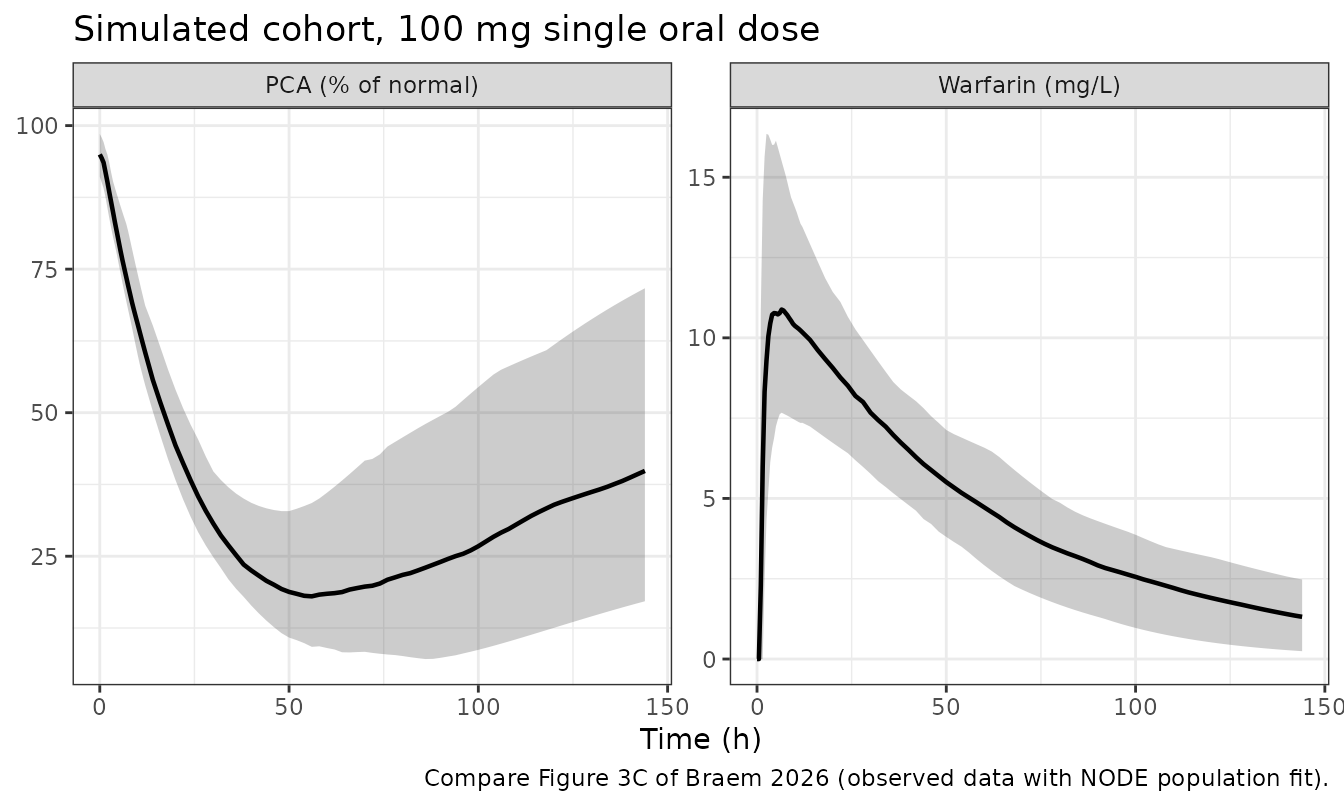

The paper reports no NCA values for warfarin, so the NCA below is checked against the quantity the model itself determines: for a linear one-compartment oral model with complete bioavailability, AUC(0-inf) = Dose / CL.

sim_nca <- sim |>
  filter(!is.na(Cc)) |>
  select(id, time, Cc, treatment)

sim_nca <- bind_rows(
  sim_nca,
  sim_nca |> distinct(id, treatment) |> mutate(time = 0, Cc = 0)
) |>
  distinct(id, treatment, time, .keep_all = TRUE) |>
  arrange(id, treatment, time)

conc_obj <- PKNCA::PKNCAconc(sim_nca, Cc ~ time | treatment + id)

dose_df  <- cohort_ev |>
  filter(evid == 1) |>
  select(time, amt, treatment) |>
  tidyr::crossing(id = unique(sim_nca$id))
dose_obj <- PKNCA::PKNCAdose(dose_df, amt ~ time | treatment + id)

nca_res <- PKNCA::pk.nca(PKNCA::PKNCAdata(
  conc_obj, dose_obj,
  intervals = data.frame(start = 0, end = Inf,
                         cmax = TRUE, tmax = TRUE,
                         aucinf.obs = TRUE, half.life = TRUE)
))

nca_wide <- as.data.frame(nca_res) |>
  select(id, PPTESTCD, PPORRES) |>
  pivot_wider(names_from = PPTESTCD, values_from = PPORRES)

nca_summary <- nca_wide |>
  summarise(across(c(cmax, tmax, aucinf.obs, half.life),
                   list(median = ~median(.x, na.rm = TRUE)),
                   .names = "{.col}"))

cl_typical  <- exp(ini_w[["lcl"]])
auc_expected <- 100 / cl_typical

tibble::tibble(
  `NCA parameter` = c("Cmax (mg/L)", "Tmax (h)", "AUC0-inf (mg*h/L)", "t1/2 (h)"),
  `Simulated median` = c(nca_summary$cmax, nca_summary$tmax,
                         nca_summary$aucinf.obs, nca_summary$half.life),
  `Model-implied reference` = c(NA, NA, auc_expected, log(2) / (cl_typical / exp(ini_w[["lvc"]])))
) |>
  knitr::kable(digits = 2,
               caption = "Simulated NCA vs the values the packaged PK parameters imply.")

Simulated NCA vs the values the packaged PK parameters imply.
NCA parameter	Simulated median	Model-implied reference
Cmax (mg/L)	11.11	NA
Tmax (h)	4.25	NA
AUC0-inf (mg*h/L)	752.35	764.54
t1/2 (h)	42.99	42.41

auc_pct <- 100 * (nca_summary$aucinf.obs - auc_expected) / auc_expected
auc_pct
#> [1] -1.593756

# Cohort-derived, so bound the magnitude with headroom rather than pinning a
# value from one draw. The median of a log-normal AUC is Dose/CL exactly, so
# the residual is not a distributional offset: it is `aucinf.obs` tail
# extrapolation. Observations stop at 144 h, only about 3.4 terminal
# half-lives, so a large extrapolated fraction is fitted from a log-linear
# slope that the simulated cohort reads slightly long (44.7 h vs the
# model-implied 42.4 h) -- which inflates AUC. The residual is also strongly
# cohort-dependent, because rxode2 partitions its RNG streams per solver
# thread: realised +4.73% at 16 threads and -1.59% at 2. Do not tighten to
# either. A mis-transcribed dose, volume or clearance moves this by tens of
# percent, so 15 still goes red for the failures that matter.
stopifnot(abs(auc_pct) < 15)

Part 2 – the automatically-proposed bi-exponential model

The LASSO step selected a linear function of amount plus an exponential function of time, giving (Equation 20)

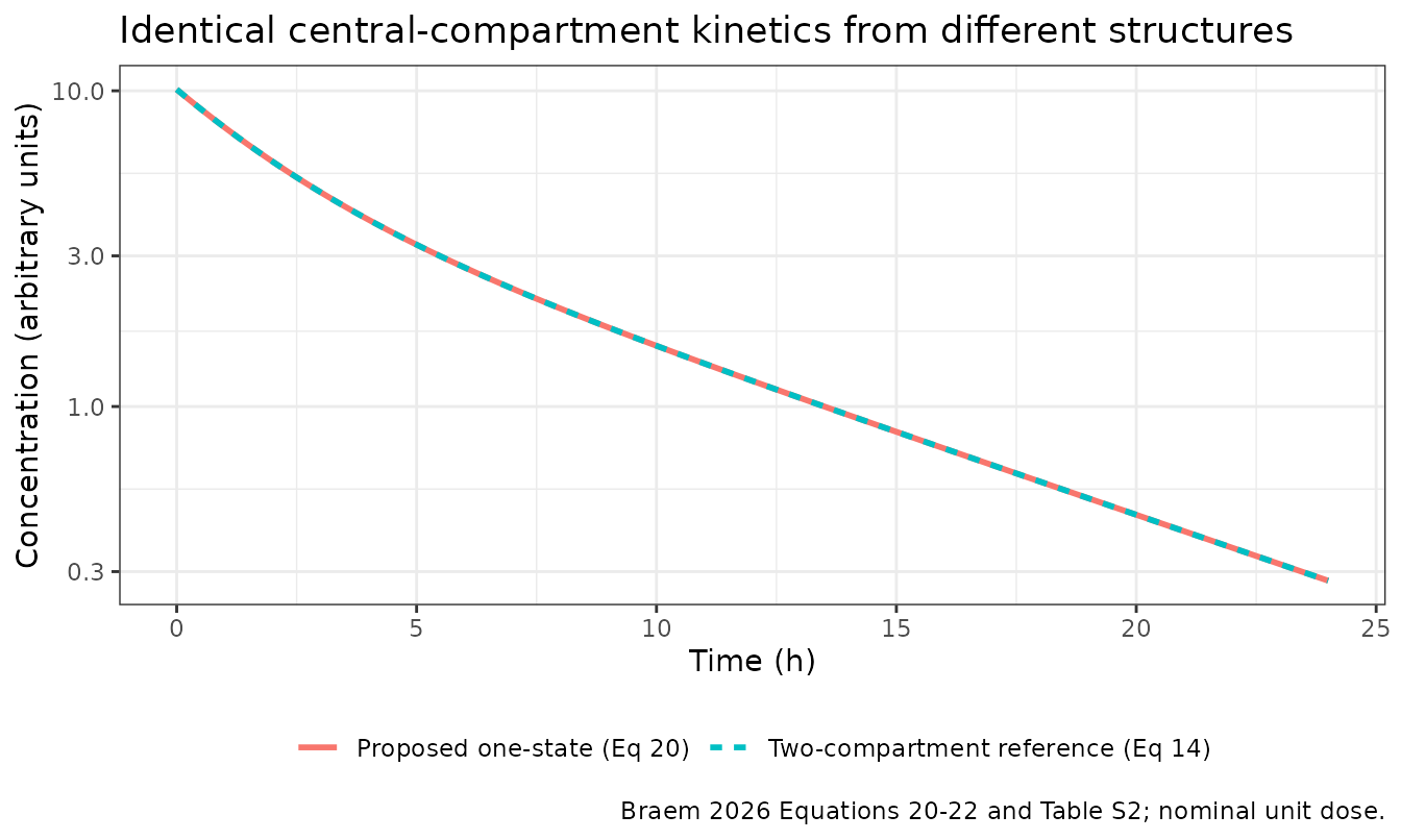
$\frac{dA_C}{dt} = -k_{el} A_C - D \cdot w_{dist}\, e^{-k_{dist} t}, \qquad A_C(0) = D, \qquad C_C = A_C / V_c .$

There is no peripheral compartment. The paper’s claim – and the reason the example is interesting – is that this single-state model has an explicit solution identical to the central compartment of the two-compartment model that generated the data.

Recovering the parameters from Table S2

Braem 2026 never prints the estimates of Equation 20. Table S2 gives the macro-parameters of its explicit solution (Equation 21), Cc(t) = A' exp(-kdist t) + B' exp(-kel t), together with kel and kdist themselves. The paper’s own definitions of A' and B' then invert exactly.

Ap <- 5.1; kdist <- 0.46; Bp <- 5.0; kel <- 0.12   # Table S2

# A' = -(D/Vc) * wdist / (kel - kdist);  B' = (D/Vc) * (kel - kdist + wdist) / (kel - kdist)
# Summing telescopes the bracket:  A' + B' = D/Vc.
d_over_v <- Ap + Bp
wdist    <- Ap * (kel - kdist) / -d_over_v

c(`D/Vc` = d_over_v, wdist = wdist)
#>       D/Vc      wdist 
#> 10.1000000  0.1716832

# Round-trip the inversion back through the paper's own formulas.
stopifnot(
  abs(-d_over_v * wdist / (kel - kdist) - Ap) < 1e-9,
  abs(d_over_v * (kel - kdist + wdist) / (kel - kdist) - Bp) < 1e-9
)

# And the standard macro-to-micro inversion for the two-compartment reference.
A <- 5.1; alpha <- 0.46; B <- 5.0; beta <- 0.12    # Table S2
k21 <- (A * beta + B * alpha) / (A + B)
k10 <- alpha * beta / k21
k12 <- alpha + beta - k10 - k21
vc2 <- 1 / (A + B)

stopifnot(
  abs((k10 + k12 + k21) - (alpha + beta)) < 1e-12,
  abs(k10 * k21 - alpha * beta) < 1e-12
)
c(vc = vc2, cl = k10 * vc2, q = k12 * vc2, vp = k12 * vc2 / k21)
#>          vc          cl           q          vp 
#> 0.099009901 0.018956044 0.009923478 0.034418655

The fit identifies the model only up to the ratio D/Vc = 10.1; the dose was never reported. Both packaged models therefore fix a nominal unit dose, so vc = 1/10.1, and a dose of 1 arbitrary unit reproduces Table S2 exactly. The model is linear, so any other dose scales the profile exactly.

Gates 3-5 – both models against their closed forms, and against each other

biexp_ev <- rxode2::et(amt = 1, cmt = "central") |>
  rxode2::et(seq(0, 24, by = 0.1))

sim_prop <- rxode2::rxSolve(uis[["Bram_2026_biexponential"]], biexp_ev,
                            returnType = "data.frame")
sim_2cmt <- rxode2::rxSolve(uis[["Bram_2026_biexponential_2cmt"]], biexp_ev,
                            returnType = "data.frame")

closed_form <- 5.1 * exp(-0.46 * sim_prop$time) + 5.0 * exp(-0.12 * sim_prop$time)

gates <- c(
  `proposed vs Eq 21` = max(abs(sim_prop$Cc - closed_form) / closed_form),
  `2-cmt vs Eq 22`    = max(abs(sim_2cmt$Cc - closed_form) / closed_form),
  `proposed vs 2-cmt` = max(abs(sim_prop$Cc - sim_2cmt$Cc) / sim_2cmt$Cc)
)
gates
#> proposed vs Eq 21    2-cmt vs Eq 22 proposed vs 2-cmt 
#>      4.655206e-07      6.595467e-07      6.384738e-07

# These are deterministic solves of published constants against a published
# closed form -- no cohort, no RNG -- so a tight bound is correct and is what
# catches a regression. Realised ~5e-07.
stopifnot(all(gates < 1e-4))

That third number is the paper’s central structural claim, reproduced: a model with no peripheral compartment and a model with one give the same central-compartment concentration to seven significant figures.

PKNCA on the pair

biexp_conc <- bind_rows(
  tibble(id = 1L, time = sim_prop$time, Cc = sim_prop$Cc,
         model = "Proposed one-state"),
  tibble(id = 1L, time = sim_2cmt$time, Cc = sim_2cmt$Cc,
         model = "Two-compartment")
) |>
  filter(!is.na(Cc)) |>
  arrange(model, id, time)

biexp_dose <- tibble(id = 1L, time = 0, amt = 1,
                     model = unique(biexp_conc$model))

biexp_nca <- PKNCA::pk.nca(PKNCA::PKNCAdata(
  PKNCA::PKNCAconc(biexp_conc, Cc ~ time | model + id),
  PKNCA::PKNCAdose(biexp_dose, amt ~ time | model + id),
  intervals = data.frame(start = 0, end = Inf,
                         cmax = TRUE, tmax = TRUE,
                         aucinf.obs = TRUE, half.life = TRUE)
))

# Table S2 fixes AUC(0-inf) analytically: A/alpha + B/beta.
auc_published <- A / alpha + B / beta

biexp_tab <- as.data.frame(biexp_nca) |>
  select(model, PPTESTCD, PPORRES) |>
  pivot_wider(names_from = PPTESTCD, values_from = PPORRES)

biexp_tab |>
  mutate(`AUC from Table S2` = auc_published,
         `AUC % diff` = 100 * (aucinf.obs - auc_published) / auc_published) |>
  rename("Model" = model, "Cmax" = cmax, "Tmax (h)" = tmax,
         "AUC0-inf" = aucinf.obs, "t1/2 (h)" = half.life) |>
  knitr::kable(digits = 4,
               caption = "NCA of both models vs the AUC that Table S2 determines analytically.")

NCA of both models vs the AUC that Table S2 determines analytically.
Model	Cmax	Tmax (h)	tlast	clast.obs	lambda.z	r.squared	adj.r.squared	lambda.z.time.first	lambda.z.time.last	lambda.z.n.points	clast.pred	t1/2 (h)	span.ratio	AUC0-inf	AUC from Table S2	AUC % diff
Proposed one-state	10.1	0	24	0.2808	0.122	0.9999	0.9999	9.5	24	146	0.2788	5.6799	2.5529	52.7158	52.7536	-0.0717
Two-compartment	10.1	0	24	0.2808	0.122	0.9999	0.9999	9.5	24	146	0.2788	5.6799	2.5529	52.7158	52.7536	-0.0716


# Deterministic solve + trapezoidal NCA on a 0.1 h grid; realised < 0.05%.
stopifnot(
  max(abs(100 * (biexp_tab$aucinf.obs - auc_published) / auc_published)) < 1,
  # Both models must give the same Cmax: it is the same profile.
  diff(range(biexp_tab$cmax)) < 1e-4
)

Gate 6 – the documented multiple-dose limitation

Braem 2026 Figure S1 shows that the proposed one-state model is structurally misspecified when a dose arrives before the previous distribution phase has finished, because the model carries no memory of earlier doses. That is a property of the model, not a defect of this encoding, and it is worth demonstrating so a user does not walk into it.

compare_regimen <- function(ii, n_doses) {
  ev <- rxode2::et(amt = 1, cmt = "central", ii = ii, addl = n_doses - 1L) |>
    rxode2::et(seq(0, ii * n_doses, by = 0.1))
  p <- rxode2::rxSolve(uis[["Bram_2026_biexponential"]], ev, returnType = "data.frame")
  r <- rxode2::rxSolve(uis[["Bram_2026_biexponential_2cmt"]], ev, returnType = "data.frame")
  max(abs(p$Cc - r$Cc) / pmax(r$Cc, 1e-8))
}

multidose <- c(
  `q24h (dose after distribution phase)` = compare_regimen(24, 4L),
  `q2h  (dose within distribution phase)` = compare_regimen(2, 12L)
)
multidose
#>  q24h (dose after distribution phase) q2h  (dose within distribution phase) 
#>                          1.857452e-05                          2.700860e-01

# Deterministic. The q24h agreement is the paper's stated validity condition;
# the q2h disagreement is the Figure S1 misspecification, and asserting that it
# is LARGE is what stops a future refactor from silently "fixing" the model
# into something the paper did not publish.
stopifnot(
  multidose[[1]] < 0.05,
  multidose[[2]] > 0.20
)

Assumptions and deviations

No parameter table exists in the article. Every value in all three models comes from the Supporting Information (Table S2) or from the authored Data S2 code deposit. This is recorded per parameter in the model files and in the source-trace table above.
Warfarin NODE parameters are non-paper-derived. All 21 estimates and both residual-error models come from the deposited Monolix run Warf_node_mlx_file_ind (populationParameters.txt and the .mlxtran DEFINITION block). The deposit contains two runs; the one used here is the final one, with IIV on the network parameters, which is the fit whose MARE the article reports.
Monolix omega is a standard deviation; nlmixr2 takes a variance. Every IIV entry in the warfarin model is the deposited omega squared, noted inline.
The additive residual SD on Cc collapsed to zero. The deposit reports acp = 2.22e-16, the optimiser’s lower bound. It is transcribed verbatim rather than dropped, so the combined1 error model matches the deposit exactly; in practice the concentration residual is effectively proportional.
The bi-exponential parameters wdist and Vc are back-solved, not printed. Table S2 gives A', B', kel and kdist; wdist and D/Vc follow exactly from the paper’s own definitions of A' and B', and the inversion is round-tripped in the vignette above.
The bi-exponential dose is unreported, so a nominal unit dose is fixed. Both bi-exponential models are identified only up to D/Vc = 10.1. Setting D = 1 gives vc = 1/10.1; the model is linear, so any other dose scales the profile exactly and nothing is invented beyond the published ratio. Units for dose and concentration are declared as placeholders (dose_unit, conc_unit) because the source data were simulated and carry none.
No IIV and no residual error for either bi-exponential model. Braem 2026 states that parameters were assumed log-normally distributed but reports no omega and no sigma for Equations 14 or 20. Nothing is invented; both models are typical-value only.
Two of the paper’s models are not packaged. The neonatal weight model (Equation 18) and the LASSO-distilled warfarin model (Equation 24) report no final estimates anywhere on disk. See the coverage table above for why the Figure 4 panels do not rescue them.
podo() and tad() need their compartment argument. In Bram_2026_biexponential, the transient flux is written podo(central) * wdist * exp(-kdist * tad(central)). Verified on rxode2 5.1.7: through the rxUi path that readModelDb() and rxSolve() use, the argument-less podo() / tad() silently evaluate to zero, which drops the term and degrades the model to a mono-exponential with no warning. Gate 3 above exists to catch exactly that regression.