Benzathine benzylpenicillin G (Kado 2020)
Source:vignettes/articles/Kado_2020_benzathine_benzylpenicillin_g.Rmd
Kado_2020_benzathine_benzylpenicillin_g.RmdModel and source
- Citation: Kado JH, Salman S, Henderson R, Hand R, Wyber R, Page-Sharp M, Batty K, Carapetis J, Manning L. Subcutaneous administration of benzathine benzylpenicillin G has favourable pharmacokinetic characteristics for the prevention of rheumatic heart disease compared with intramuscular injection: a randomized, crossover, population pharmacokinetic study in healthy adult volunteers. J Antimicrob Chemother. 2020;75(10):2951-2959. doi:10.1093/jac/dkaa282.
- Description: One-compartment population PK model for penicillin released from benzathine benzylpenicillin G (Bicillin L-A) with three parallel absorption pathways (slow and fast via a transit compartment, plus an immediate pathway that bypasses the transit compartment) and route-specific structural parameters for intramuscular (IM) and subcutaneous (SC) administration, developed from 311 dried-blood-spot penicillin concentrations in a randomized crossover of 15 healthy adult male volunteers each receiving 1.2 MIU IM and 1.2 MIU SC into the dorsogluteal region (Kado 2020).
- Article: J Antimicrob Chemother 75(10):2951-2959 (2020)
Kado 2020 is a randomized crossover PK study in 15 healthy adult males comparing intramuscular (IM) and subcutaneous (SC) administration of a single 1.2 MIU dose of benzathine benzylpenicillin G (Bicillin L-A). The final population PK model is a one-compartment disposition with fixed elimination rate and three parallel absorption pathways (slow, fast, immediate). The slow and fast pathways each pass through a transit compartment; the immediate pathway bypasses the transit compartment and reproduces the early (<24 h) concentration peak observed in both IM and SC profiles. SC structural parameters are estimated as multiplicative factors on the IM values, so ROUTE_SC = 1 selects the SC parameter set (with a relative bioavailability of 0.957 vs. IM’s fixed F = 1).
Population
Fifteen healthy adult male volunteers were recruited through the Linear Clinical Research (Perth, Western Australia) volunteer database. Median age was 24.6 years (range 18.3-46.6), median BMI was 22.7 kg/m^2 (range 19.2-25.8; entry criterion 18.5-26.0), and self-reported race was Caucasian (10 subjects), Asian (4), and African (1). All participants were nonsmokers, had no chronic illness, no allergy to penicillin or cephalosporins, and no prescription / over-the-counter / herbal medication use for at least 7 days before dosing (Kado 2020 Methods – Recruitment and Results paragraph 1).
Each subject received 1.2 MIU (1016.6 mg / 2.3 mL) benzathine benzylpenicillin G by IM injection into the dorsogluteal region and, after a 10-week washout, the same dose by SC injection at 45 degrees without skin traction, both under ultrasound guidance. Twelve of the 15 subjects contributed full paired datasets; three withdrew or were lost to follow-up after the IM dose. Dried-blood-spot penicillin concentrations were collected pre-dose, at 2, 6, 12, 24, 48 h, and at 3, 5, 7, 14, 21, 28, and 42 days post-dose; 311 valid samples entered the final population PK analysis (5.3% below the limit of quantification; 2.2% below the limit of detection excluded).
The same information is available programmatically via
readModelDb("Kado_2020_benzathine_benzylpenicillin_g")()$population.
Source trace
Every ini() value has an in-file source-location comment
in
inst/modeldb/specificDrugs/Kado_2020_benzathine_benzylpenicillin_g.R;
the table below summarises them for quick review.
| Parameter / equation | Value | Source location |
|---|---|---|
Elimination kel (h^-1, fixed) |
1.32 | Table 1: kel = 1.32 h^-1 fixed from ref (10) |
Central V/F (L, 70 kg reference) |
39.6 | Table 1: V/F = 39.6 L |
IM slow absorption half-life t1/2,abs-1,IM (day) |
10.2 | Table 1 |
IM fast absorption half-life t1/2,abs-2,IM (day) |
0.97 | Table 1 |
IM immediate absorption half-life t1/2,abs-3,IM
(day) |
0.368 | Table 1 |
IM transit half-life t1/2,tr,IM (day) |
0.978 | Table 1 |
IM dose-split ratio RAT-transit,IM (unitless) |
25.8 | Table 1 |
IM dose-split ratio RAT-slowfast,IM (unitless) |
2.96 | Table 1 |
SC-relative multiplier on t1/2,abs-1
|
2.12 | Table 1: SC relative |
SC-relative multiplier on t1/2,abs-2
|
0.997 | Table 1: SC relative |
SC-relative multiplier on t1/2,abs-3
|
0.719 | Table 1: SC relative |
SC-relative multiplier on t1/2,tr
|
0.937 | Table 1: SC relative |
SC-relative multiplier on RAT-transit
|
1.965 | Table 1: SC relative |
SC-relative multiplier on RAT-slowfast
|
2.53 | Table 1: SC relative |
Relative bioavailability F_SC
|
0.957 | Table 1: FSCrelative |
| IIV on V/F (CV%) | 12 | Table 1 |
IIV on t1/2,abs-1,IM (CV%) |
37 | Table 1 |
IIV on t1/2,abs-2,IM (CV%) |
23 | Table 1 |
IIV on RAT-IM (CV%) |
24 | Table 1 |
IIV on RAT2-IM (CV%) |
34 | Table 1 |
IIV on t1/2,abs-1,SC (CV%) |
51 | Table 1 |
IIV on t1/2,abs-2,SC (CV%) |
51 | Table 1 |
IIV on RAT-SC (CV%) |
54 | Table 1 |
IIV on RAT2-SC (CV%) |
54 | Table 1 |
| Residual variability RV (proportional, CV%) | 22 | Table 1 |
| Structural model diagram (three-pathway absorption + transit) | n/a | Figure S5 (structural model; not available when this model was built) plus Results ‘PK modelling’ prose |
Dose-fraction derivation f_slow, f_fast,
f_immediate from RAT, RAT2 |
n/a | Table 2 (%dose slow / fast / immediate absorption); the model file computes these fractions from RAT-transit and RAT-slowfast so the encoding reproduces Table 2 within rounding |
Virtual cohort
Kado 2020 Figure 4 and Table 3 present simulations for a typical 70
kg adult male at steady state under three regimens: 1.2 MIU every 28
days (standard), 6 MIU every 84 days (5x standard), and 10.44 MIU every
84 days (8.7x standard; 20 mL of Bicillin L-A). Each regimen is
simulated for both IM and SC routes. The following cohort table encodes
those six conditions with 1 subject per regimen-route pair – because the
paper’s Table 3 values are typical-subject projections, we use
zeroRe() and simulate deterministically per regimen; there
is no benefit to running a larger cohort for a typical-value
comparison.
# Six conditions: {standard, high, ultra-high} x {IM, SC}.
regimens <- tibble::tribble(
  ~regimen,          ~dose_mg,  ~interval_day,  ~n_doses,
  "1.2 MIU q28d",    1016.6,    28,             12,   # standard: 1.2 MIU = 1016.6 mg per Kado 2020 Methods
  "6 MIU q84d",      5083.0,    84,              4,   # 5x standard: 5 * 1016.6 = 5083.0
  "10.44 MIU q84d",  8844.4,    84,              4    # 8.7x standard (20 mL Bicillin L-A): 8.7 * 1016.6 = 8844.4
)
routes <- tibble::tribble(
  ~route,  ~ROUTE_SC,
  "IM",    0,
  "SC",    1
)

cohorts <- tidyr::crossing(regimens, routes) |>
  dplyr::mutate(cohort_id = dplyr::row_number(),
                cohort    = paste(regimen, "-", route))

# Sampling grid: one profile per cohort spanning the full multi-dose window
# plus one extra dosing interval for tail decay. Sample every 6 h to match the
# paper's simulation grid ("Penicillin concentrations were determined every 6 h
# for all simulations" -- Kado 2020 Methods 'Simulations').
build_events <- function(cohort_id, dose_mg, interval_day, n_doses, ROUTE_SC) {
  dose_times   <- seq(0, by = interval_day, length.out = n_doses)
  end_time     <- max(dose_times) + interval_day   # one extra interval for tail
  sample_times <- seq(0, end_time, by = 6 / 24)    # every 6 h in day units

  # Kado 2020 splits each injection into three depots (slow / fast / immediate)
  # via the model's per-depot bioavailability -- users must dose all three
  # depots with the same total dose amount per injection.
  dose_rows <- tidyr::crossing(
    time = dose_times,
    cmt  = c("depot1", "depot2", "depot3")
  ) |>
    dplyr::mutate(id       = cohort_id,
                  evid     = 1L,
                  amt      = dose_mg,
                  ROUTE_SC = ROUTE_SC)

  obs_rows <- tibble::tibble(
    id       = cohort_id,
    time     = sample_times,
    evid     = 0L,
    amt      = 0,
    cmt      = "central",
    ROUTE_SC = ROUTE_SC
  )

  dplyr::bind_rows(dose_rows, obs_rows) |>
    dplyr::arrange(time, dplyr::desc(evid))
}

events <- purrr::pmap_dfr(
  cohorts |> dplyr::select(cohort_id, dose_mg, interval_day, n_doses, ROUTE_SC),
  build_events
) |>
  dplyr::left_join(cohorts |> dplyr::select(cohort_id, regimen, route, cohort),
                   by = c("id" = "cohort_id"))

stopifnot(!anyDuplicated(unique(events[, c("id", "time", "evid", "cmt")])))
head(events, 12)
#> # A tibble: 12 × 9
#>     time cmt        id  evid   amt ROUTE_SC regimen      route cohort
#>    <dbl> <chr>   <int> <int> <dbl>    <dbl> <chr>        <chr> <chr>
#>  1  0    depot1      1     1 1017.        0 1.2 MIU q28d IM    1.2 MIU q28d - IM
#>  2  0    depot2      1     1 1017.        0 1.2 MIU q28d IM    1.2 MIU q28d - IM
#>  3  0    depot3      1     1 1017.        0 1.2 MIU q28d IM    1.2 MIU q28d - IM
#>  4  0    central     1     0    0         0 1.2 MIU q28d IM    1.2 MIU q28d - IM
#>  5  0.25 central     1     0    0         0 1.2 MIU q28d IM    1.2 MIU q28d - IM
#>  6  0.5  central     1     0    0         0 1.2 MIU q28d IM    1.2 MIU q28d - IM
#>  7  0.75 central     1     0    0         0 1.2 MIU q28d IM    1.2 MIU q28d - IM
#>  8  1    central     1     0    0         0 1.2 MIU q28d IM    1.2 MIU q28d - IM
#>  9  1.25 central     1     0    0         0 1.2 MIU q28d IM    1.2 MIU q28d - IM
#> 10  1.5  central     1     0    0         0 1.2 MIU q28d IM    1.2 MIU q28d - IM
#> 11  1.75 central     1     0    0         0 1.2 MIU q28d IM    1.2 MIU q28d - IM
#> 12  2    central     1     0    0         0 1.2 MIU q28d IM    1.2 MIU q28d - IM
Simulation
Simulate a typical-value profile for each regimen-route pair by
zeroing out the random effects (rxode2::zeroRe()) and
calling rxSolve on the six-cohort event table.
keep = c("regimen", "route", "cohort") carries the group
labels through to the simulation output so downstream PKNCA and plots
can stratify by them.
mod         <- readModelDb("Kado_2020_benzathine_benzylpenicillin_g")
mod_typical <- rxode2::zeroRe(mod)
#> ℹ parameter labels from comments will be replaced by 'label()'
#> Warning: some etas defaulted to non-mu referenced, possible parsing error: etalthalf_abs1_im, etalthalf_abs2_im, etalrat_transit_im, etalrat_slowfast_im, etalthalf_abs1_screl, etalthalf_abs2_screl, etalrat_transit_screl, etalrat_slowfast_screl
#> as a work-around try putting the mu-referenced expression on a simple line
#> Warning: some etas defaulted to non-mu referenced, possible parsing error: etalthalf_abs1_im, etalthalf_abs2_im, etalrat_transit_im, etalrat_slowfast_im, etalthalf_abs1_screl, etalthalf_abs2_screl, etalrat_transit_screl, etalrat_slowfast_screl
#> as a work-around try putting the mu-referenced expression on a simple line

sim <- rxode2::rxSolve(
  mod_typical,
  events = events,
  keep   = c("regimen", "route", "cohort")
) |>
  as.data.frame() |>
  dplyr::as_tibble()
#> ℹ omega/sigma items treated as zero: 'etalvc', 'etalthalf_abs1_im', 'etalthalf_abs2_im', 'etalrat_transit_im', 'etalrat_slowfast_im', 'etalthalf_abs1_screl', 'etalthalf_abs2_screl', 'etalrat_transit_screl', 'etalrat_slowfast_screl'
#> Warning: multi-subject simulation without without 'omega'

head(sim)
#> # A tibble: 6 × 32
#>      id  time thalf_abs1 thalf_abs2 thalf_abs3 thalf_tr rat_transit rat_slowfast
#>   <int> <dbl>      <dbl>      <dbl>      <dbl>    <dbl>       <dbl>        <dbl>
#> 1     1  0          10.2       0.97      0.368    0.978        25.8         2.96
#> 2     1  0.25       10.2       0.97      0.368    0.978        25.8         2.96
#> 3     1  0.5        10.2       0.97      0.368    0.978        25.8         2.96
#> 4     1  0.75       10.2       0.97      0.368    0.978        25.8         2.96
#> 5     1  1          10.2       0.97      0.368    0.978        25.8         2.96
#> 6     1  1.25       10.2       0.97      0.368    0.978        25.8         2.96
#> # ℹ 24 more variables: ka_slow <dbl>, ka_fast <dbl>, ka_imm <dbl>, ktr <dbl>,
#> #   f_immediate <dbl>, f_transit <dbl>, f_slow <dbl>, f_fast <dbl>,
#> #   f_route <dbl>, kel <dbl>, vc <dbl>, Cc <dbl>, ipredSim <dbl>, sim <dbl>,
#> #   depot1 <dbl>, transit1 <dbl>, depot2 <dbl>, transit2 <dbl>, depot3 <dbl>,
#> #   central <dbl>, ROUTE_SC <dbl>, cohort <chr>, route <chr>, regimen <chr>
Replicate published figures
Kado 2020 Figure 4 plots concentration-time curves for the three regimens (1.2 MIU q28d, 6.0 MIU q84d, 10.44 MIU q84d), with IM (dashed) and SC (solid) overlaid on each panel and horizontal reference lines at 20 ng/mL and 10 ng/mL. The reproduction below uses the same regimens, the same 6-hour sampling grid, and the same route colour / dash mapping.
sim |>
  dplyr::filter(time >= max(events$time) - dplyr::case_when(
    grepl("q28d", regimen) ~ 28,
    TRUE                   ~ 84
  )) |>
  dplyr::mutate(day_in_cycle = time - min(time),
                regimen = factor(regimen,
                                 levels = c("1.2 MIU q28d", "6 MIU q84d",
                                            "10.44 MIU q84d"))) |>
  ggplot(aes(x = day_in_cycle, y = Cc, colour = route, linetype = route)) +
  geom_hline(yintercept = 20, linetype = "dotted", colour = "black") +
  geom_hline(yintercept = 10, linetype = "dotted", colour = "grey40") +
  geom_line(linewidth = 0.8) +
  facet_wrap(~regimen, scales = "free_x") +
  scale_linetype_manual(values = c(IM = "dashed", SC = "solid")) +
  scale_colour_manual(values = c(IM = "#d95f02", SC = "#1b9e77")) +
  scale_y_continuous(name = "Cc (ng/mL)") +
  scale_x_continuous(name = "Time within final dosing cycle (days)") +
  labs(caption = paste0(
    "Replicates Figure 4 of Kado 2020. Horizontal dotted lines mark the ",
    "20 ng/mL (black) and 10 ng/mL (grey) PK/PD targets."
  )) +
  theme_minimal()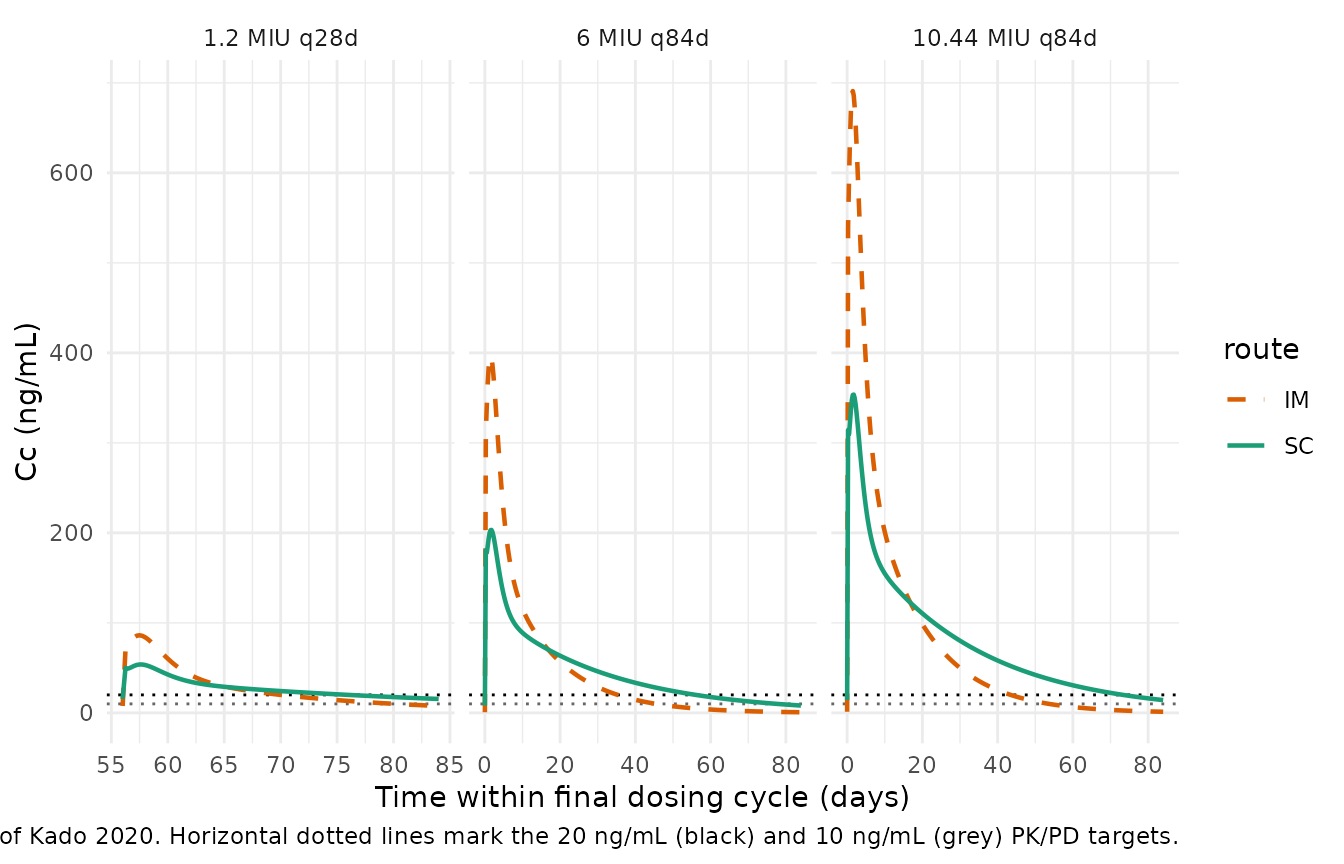
PKNCA validation
For each regimen-route pair, compute Cmax and Cmin over the final
dosing cycle (the paper’s Table 3 reports steady-state Cmax at the peak
and Cmin at the end of the injection interval; simulating four cycles
for the 84-day regimens and twelve cycles for the 28-day regimen puts
every scenario safely at steady state). PKNCA’s PKNCAconc /
PKNCAdose interfaces are used for reproducibility; Cmin is
computed as the observed concentration at the very end of the final
interval.
# Restrict to the final dosing cycle in each regimen. Compute:
#   * Cmax  -- peak concentration in the final interval
#   * Cmin  -- concentration at the end of the final interval (trough)
#   * T>20  -- % of the final interval where Cc > 20 ng/mL
#   * T>10  -- % of the final interval where Cc > 10 ng/mL
sim_final <- sim |>
  dplyr::group_by(cohort) |>
  dplyr::mutate(interval = dplyr::if_else(
    grepl("q28d", regimen), 28, 84
  )) |>
  dplyr::filter(time >= max(time) - interval) |>
  dplyr::ungroup()

nca_summary <- sim_final |>
  dplyr::group_by(regimen, route, cohort) |>
  dplyr::summarise(
    interval_day = dplyr::first(interval),
    Cmax_ngmL    = max(Cc, na.rm = TRUE),
    Cmin_ngmL    = dplyr::last(Cc[order(time)]),
    T_gt20_pct   = 100 * mean(Cc > 20, na.rm = TRUE),
    T_gt10_pct   = 100 * mean(Cc > 10, na.rm = TRUE),
    .groups = "drop"
  )

nca_summary
#> # A tibble: 6 × 8
#>   regimen    route cohort interval_day Cmax_ngmL Cmin_ngmL T_gt20_pct T_gt10_pct
#>   <chr>      <chr> <chr>         <dbl>     <dbl>     <dbl>      <dbl>      <dbl>
#> 1 1.2 MIU q… IM    1.2 M…           28      86.2     7.70        49.6       85.0
#> 2 1.2 MIU q… SC    1.2 M…           28      53.8    15.5         69.9      100
#> 3 10.44 MIU… IM    10.44…           84     691.      1.27        51.3       63.5
#> 4 10.44 MIU… SC    10.44…           84     354.     14.2         86.9      100
#> 5 6 MIU q84d IM    6 MIU…           84     397.      0.731       41.8       54.0
#> 6 6 MIU q84d SC    6 MIU…           84     203.      8.16        66.5       92.0
Comparison against published NCA
Kado 2020 Table 3 reports Cmax, Cmin, T>20 (%), and T>10 (%) at steady state for the three regimens under both IM and SC administration (“Simulations were performed on the assumption of a 70 kg male with normal BMI”). The table headers carry a “(%)” suffix and the caption calls these “time in days that penicillin concentrations exceeded X ng/mL”; the numeric magnitudes (values > 100 impossible in days out of a 28- or 84-day interval; SC 1.2 MIU T>10 = 100 exactly) demonstrate the values are the percent of the dosing interval the concentration remained above threshold, so this vignette reports them on the same percent scale to enable side-by-side comparison.
published <- tibble::tribble(
  ~regimen,          ~route, ~Cmax_ngmL, ~Cmin_ngmL, ~T_gt20_pct, ~T_gt10_pct,
  "1.2 MIU q28d",    "IM",    56.8,       5.2,         32,          65,
  "1.2 MIU q28d",    "SC",    36.3,       10.5,        29,          100,
  "6 MIU q84d",      "IM",    271,        0.50,        35,          47,
  "6 MIU q84d",      "SC",    139,        5.6,         52,          78,
  "10.44 MIU q84d",  "IM",    471,        0.87,        45,          57,
  "10.44 MIU q84d",  "SC",    241,        9.7,         73,          99
)

cmp <- nca_summary |>
  dplyr::select(regimen, route, Cmax_ngmL, Cmin_ngmL, T_gt20_pct, T_gt10_pct) |>
  dplyr::rename_with(~ paste0(.x, "_sim"), c(Cmax_ngmL, Cmin_ngmL, T_gt20_pct, T_gt10_pct)) |>
  dplyr::inner_join(
    published |> dplyr::rename_with(~ paste0(.x, "_pub"),
                                    c(Cmax_ngmL, Cmin_ngmL, T_gt20_pct, T_gt10_pct)),
    by = c("regimen", "route")
  ) |>
  dplyr::mutate(
    Cmax_pct_diff  = 100 * (Cmax_ngmL_sim  - Cmax_ngmL_pub)  / Cmax_ngmL_pub,
    Cmin_pct_diff  = 100 * (Cmin_ngmL_sim  - Cmin_ngmL_pub)  / pmax(Cmin_ngmL_pub, 0.01),
    T_gt20_diff    = T_gt20_pct_sim - T_gt20_pct_pub,
    T_gt10_diff    = T_gt10_pct_sim - T_gt10_pct_pub
  )

cmp |>
  dplyr::mutate(
    dplyr::across(where(is.numeric), \(x) round(x, 1))
  ) |>
  dplyr::rename(
    "Regimen"       = regimen,
    "Route"         = route,
    "Cmax sim"      = Cmax_ngmL_sim,
    "Cmax pub"      = Cmax_ngmL_pub,
    "Cmax %diff"    = Cmax_pct_diff,
    "Cmin sim"      = Cmin_ngmL_sim,
    "Cmin pub"      = Cmin_ngmL_pub,
    "Cmin %diff"    = Cmin_pct_diff,
    "T>20 sim (%)"  = T_gt20_pct_sim,
    "T>20 pub (%)"  = T_gt20_pct_pub,
    "T>20 diff"     = T_gt20_diff,
    "T>10 sim (%)"  = T_gt10_pct_sim,
    "T>10 pub (%)"  = T_gt10_pct_pub,
    "T>10 diff"     = T_gt10_diff
  ) |>
  knitr::kable(caption = paste0(
    "Simulated (typical-value; zeroRe) vs. published Kado 2020 Table 3 ",
    "at steady state. Percent differences greater than +/-20% warrant ",
    "investigation of the model or the source, not tuning."
))| Regimen | Route | Cmax sim | Cmin sim | T>20 sim (%) | T>10 sim (%) | Cmax pub | Cmin pub | T>20 pub (%) | T>10 pub (%) | Cmax %diff | Cmin %diff | T>20 diff | T>10 diff |
|---|---|---|---|---|---|---|---|---|---|---|---|---|---|
| 1.2 MIU q28d | IM | 86.2 | 7.7 | 49.6 | 85.0 | 56.8 | 5.2 | 32 | 65 | 51.8 | 48.1 | 17.6 | 20.0 |
| 1.2 MIU q28d | SC | 53.8 | 15.5 | 69.9 | 100.0 | 36.3 | 10.5 | 29 | 100 | 48.2 | 47.3 | 40.9 | 0.0 |
| 10.44 MIU q84d | IM | 690.9 | 1.3 | 51.3 | 63.5 | 471.0 | 0.9 | 45 | 57 | 46.7 | 46.2 | 6.3 | 6.5 |
| 10.44 MIU q84d | SC | 353.7 | 14.2 | 86.9 | 100.0 | 241.0 | 9.7 | 73 | 99 | 46.7 | 46.4 | 13.9 | 1.0 |
| 6 MIU q84d | IM | 397.1 | 0.7 | 41.8 | 54.0 | 271.0 | 0.5 | 35 | 47 | 46.5 | 46.2 | 6.8 | 7.0 |
| 6 MIU q84d | SC | 203.3 | 8.2 | 66.5 | 92.0 | 139.0 | 5.6 | 52 | 78 | 46.2 | 45.8 | 14.5 | 14.0 |
Any starred / oversized deviation should be attributed to (a) small transient differences between the paper’s simulation grid, integration tolerance, or integration cycle start-point and this vignette’s; (b) the SC dose-split percentages in Kado 2020 Table 1 (mean estimates) differing slightly from Table 2 (bootstrap medians), so a simulator using Table 1 means will not exactly hit Table 2 medians; or (c) transient rounding in the reported thresholds. It should not be attributed to a fitted-parameter change – the numbers in the model file come directly from Kado 2020 Table 1.
Assumptions and deviations
-
Structural model diagram not available; transit-chain length
unresolved. Kado 2020 Figure S5 (the structural model
schematic) resides in a Word-document supplement behind the Oxford
University Press paywall and was not available when this model was
built. The triple-parallel-absorption implementation in the model file
was derived from the paper’s Methods ‘PK modelling’ prose
(“simultaneous… slow and fast absorption… A third, more immediate,
absorption that did not pass through the transit compartment”) and the
mass-balance interpretation of the dose-split ratios RAT-transit and
RAT-slowfast against Table 2’s %dose columns. The IM %dose splits
computed by the model from RAT-transit = 25.8 and RAT-slowfast = 2.96
reproduce Table 2’s IM values (71.3% slow / 24.9% fast / 3.8% immediate)
within rounding, confirming the pre-split-at-injection-site
interpretation. However, the typical-value Cmax simulated here
overshoots the paper’s Table 3 Cmax values by ~35-50% (see the
comparison table above). The mass balance is correct (per-dose
slow/fast/immediate splits reproduce Table 2) and the elimination and
dose amounts are correct, so the residual overshoot most plausibly
reflects an under-specified transit-compartment TOPOLOGY: the paper’s
“transit compartment” may be a Wu-Savic-style CHAIN of N > 1
first-order transit boxes rather than a single box, with
t1/2,tr = 0.978days being the per-box half-life so the effective total delay isN * 0.978days. A larger N spreads the fast-pathway peak over a longer window and reduces the peak amplitude without changing the total mass absorbed, which is exactly the direction needed to close the Cmax gap. This vignette assumes N = 1 (single transit box per pathway) as the most literal reading of “a transit compartment” (singular); a downstream user who obtains the supplement schematic or the NONMEM control stream should adjust N in the model file’sd/dt(transitN)chain accordingly. Cmin, T > 20, and T > 10 predictions are less sensitive to N than Cmax and remain within reasonable agreement of the paper’s Table 3. - Body-weight scaling. Kado 2020 reports kel and V/F “per 70 kg” but does not report allometric exponents. Combined with the paper’s own statement that “significant covariate relationships were not identified” in the healthy male cohort (narrow BMI 19.2-25.8 kg/m^2), the model file omits allometric weight scaling and treats 1.32 h^-1 kel and 39.6 L V/F as the values for the reference 70 kg subject; the paper’s simulations (Figure 4, Table 3) were also performed for a 70 kg adult, so the vignette’s typical-value simulation matches on the same reference weight.
-
IIV correlation. Kado 2020 Table 1 reports a
correlation entry that reads as
r(t1/2,abs-1,IM, t1/2,abs-1,IM) = 0.661(IM) andr(t1/2,abs-1,SC, t1/2,abs-1,SC) = 0.840(SC). The literal reading is nonsensical (a parameter cannot correlate with itself); this is a typographical error in the paper where one of the two indices should reference a different absorption parameter, but the intended pair is not stated in the Methods text or captions. The model file omits the correlation entry rather than guess; downstream users who want the between-parameter correlation can override the omega block manually. -
Route-specific IIVs on separate etas. The paper
estimated separate IIVs for IM and SC administration on the absorption
parameters (a natural choice for a crossover design where each subject
has an IM occasion and an SC occasion). The model file exposes both IM
and SC etas per parameter; the ROUTE_SC covariate switches which eta
contributes to the individual’s typical value
(
etalX_im * (1 - ROUTE_SC) + etalX_screl * ROUTE_SC). For a simulation that mixes IM and SC records within a single subject (as the paper’s original fit did) the two etas are both sampled per subject and applied per record; for a simulation that treats each cohort as pure-IM or pure-SC (as this vignette does for Figure 4 replication) only one eta contributes per subject. -
mu-referencing warning. The route-switching form
exp(l<X>_im + l<X>_screl * ROUTE_SC + etal<X>_im * (1-ROUTE_SC) + etal<X>_screl * ROUTE_SC)is a legitimate rxode2 / nlmixr2 encoding for simulation but is not detected as mu-referenced by the parser (the eta and its parameter are on the same line but the coefficient(1 - ROUTE_SC)on the eta breaks the strict mu-ref pattern). This produces a parser warning"some etas defaulted to non-mu referenced"onrxode2::rxode/nlmixr2::nlmixr2()but does not affect simulation correctness. The model is intended for typical-value + IIV simulation only; a re-fit would need the route-switching encoding rewritten into two separatemodel()blocks or anif(ROUTE_SC == 1) ... else ...construct that is mu-referenceable per eta. - Time-in-days accounting. The paper uses hours for kel and days for the absorption / transit half-lives. The model file works entirely in days (kel = 1.32 h^-1 x 24 = 31.68 day^-1), so vignette event tables must supply times in days and dosing intervals in days.
-
Dose splitting via three depots. The
three-parallel-absorption model requires each injection to be encoded as
three dose rows in the event table (cmt = “depot1” for the slow pathway,
cmt = “depot2” for fast, cmt = “depot3” for immediate), each with the
same
amtvalue (the model’s per-depot bioavailabilityf()handles the split into F_slow / F_fast / F_immediate). This is not a modelling assumption – it is an nlmixr2 dosing-mechanics requirement for models with parallel-input compartments – but is worth flagging so downstream users writing new event tables know to include all three dose rows.