Efanesoctocog alfa PK and bleed RTTE (Wong 2025)
Source:vignettes/articles/Wong_2025_efanesoctocog.Rmd
Wong_2025_efanesoctocog.RmdModel and source
Wong 2025 describes the population pharmacokinetics (PopPK) of efanesoctocog alfa, a high-sustained factor VIII (FVIII) replacement therapy for hemophilia A, and two repeated-time-to-event (RTTE) models for treated bleeding episodes. The paper estimated three models separately, and they are packaged as three files that share this vignette:
-
Wong_2025_efanesoctocog– the PopPK model: one compartment, linear elimination, body weight on CL and V, Asian race on CL. -
Wong_2025_efanesoctocog_bleed_adult– the adult/adolescent (>=12 years) bleed RTTE model from XTEND-1, with a treatment-strategy (on-demand vs prophylaxis) effect on the base hazard. -
Wong_2025_efanesoctocog_bleed_pediatric– the same structure re-estimated on children <12 years from XTEND-Kids, with no covariates.
Both RTTE files embed the PopPK model, so the hazard is driven by simulated FVIII activity exactly as in the source, where FVIII activity for each RTTE patient was predicted from the PopPK model.
- Citation: Wong N, Bhagunde P, Nyberg J, Katragadda S, Demissie M, Willemze A, Benson C, Macha S. Efanesoctocog Alfa Population Pharmacokinetics and Repeated Time-To-Event Analysis of Bleeds in Adults, Adolescents, and Children with Severe Hemophilia A. J Clin Pharmacol. 2025;65(7):860-872. doi:10.1002/jcph.70008
- Parameter tables: Tables S4 (PopPK) and S6 (RTTE) of the supplement
(
JCPH-65-860-s001.docx); the CL, V and hazard equations are in the main text.
mod_pk <- rxode2::rxode2(readModelDb("Wong_2025_efanesoctocog"))
#> ℹ parameter labels from comments will be replaced by 'label()'
mod_ad <- rxode2::rxode2(readModelDb("Wong_2025_efanesoctocog_bleed_adult"))
#> ℹ parameter labels from comments will be replaced by 'label()'
mod_pe <- rxode2::rxode2(readModelDb("Wong_2025_efanesoctocog_bleed_pediatric"))
#> ℹ parameter labels from comments will be replaced by 'label()'
Model equations
PopPK (main text, Results):
with CL in dL/h, V in dL, the dose in IU and FVIII activity in IU/dL.
Bleed hazard (main text, Results, Adult/Adolescent Model Development):
where is FVIII activity (IU/dL). In the adult/adolescent model the treatment strategy multiplies by during on-demand treatment.
Population
The PopPK model-development dataset held 3054 post-dose FVIII activity records from 260 previously treated patients with severe hemophilia A (199 adults or adolescents and 61 children <12 years; 259 male, 1 female), aged 1.4-72 years, pooled from five studies: EXTEN-A, a Phase 1 repeat-dose study, XTEND-1, XTEND-Kids and XTEND-ed (Results; Tables S1-S3). Median baseline body weight was 72.0 kg (5th-95th percentile 17.5-113 kg). The cohort was 68.1% White, 15.4% Asian and 1.9% Black, with 11.5% not reported (Table S3). All received intravenous efanesoctocog alfa, mostly 50 IU/kg once weekly.
The adult/adolescent RTTE dataset was 159 XTEND-1 patients aged 12-72 years (Table S5): 133 on once-weekly prophylaxis (Arm A) and 26 who were treated on demand for 26 weeks and then switched to once-weekly prophylaxis (Arm B). They had 361 treated bleeds, 85 in Arm A and 276 in Arm B (268 while on demand). The pediatric RTTE dataset was 74 XTEND-Kids children aged 1.4-11 years with 63 treated bleeds (Table S7).
The same information is available programmatically through each
model’s population metadata.
Source trace
| Quantity | Value | Source |
|---|---|---|
| CL at 78.3 kg, non-Asian | 0.433 dL/h | Table S4; main-text CL equation |
| V at 78.3 kg | 30.2 dL | Table S4; main-text V equation |
| Weight exponent on CL | 0.677 | Table S4 |
| Weight exponent on V | 0.791 | Table S4 |
| Asian-race factor on CL | 0.896 | Table S4; main-text CL equation |
| IIV CL, V (log-scale variance) | 0.0354, 0.0209 | Table S4 (19.0, 14.6 %CV) |
| CL-V covariance | 0.0148 | Table S4 row ‘Corr-CL-V’ |
| Proportional residual SD | 0.182 | Table S4 |
| Additive residual SD | 0.837 IU/dL | Table S4 |
| Hazard equation | Main text, Adult/Adolescent Model Development | |
| adult / pediatric | 0.00247 / 0.0000429 1/h | Table S6 |
| adult / pediatric | 1.02 / 0.694 | Table S6 |
| adult / pediatric | -1.73 / -0.00535 dL/IU | Table S6 |
| adult / pediatric | 0.247 / 1.27 | Table S6 |
| On-demand effect on (adult) | 2.21 (log scale) | Table S6 ‘Arm effect: on-demand’; Results ‘~9-fold’ |
| IIV on hazard adult / pediatric | 114 / 186 CV% -> 0.8327 / 1.4951 | Table S6; see Assumptions |
PopPK validation
Steady-state exposure for a typical patient (Table 1)
Table 1 of the paper reports the steady-state trough, peak and time above 40 IU/dL for 50 IU/kg once weekly in 1000 virtual patients at each of five fixed body weights. The typical-value prediction at each weight is a near-exact check: a one-compartment model has no other source of variation, so the typical patient should sit at the cohort median. Ten weekly doses reach steady state for every weight (the longest half-life, at 116.3 kg, is about 95 h).
wts <- c(13.4, 22.1, 50.9, 78.3, 116.3)
t_last <- 168 * 9

make_pk_events <- function(wt, id, obs_times) {
  ev <- rxode2::et(amt = 50 * wt, ii = 168, addl = 9, cmt = "central") |>
    rxode2::et(obs_times, cmt = "central") |>
    as.data.frame()
  ev$id <- id
  ev$WT <- wt
  ev$RACE_ASIAN <- 0
  ev
}

obs_ss <- seq(t_last, t_last + 168, by = 0.25)
ev_typ <- bind_rows(lapply(seq_along(wts), function(i) make_pk_events(wts[i], i, obs_ss)))

typ <- rxode2::rxSolve(rxode2::zeroRe(mod_pk), ev_typ, returnType = "data.frame") |>
  suppressWarnings() |>
  mutate(WT = wts[id])
#> ℹ omega/sigma items treated as zero: 'etalcl', 'etalvc'

typ_ss <- typ |>
  group_by(WT) |>
  summarise(
    Cmax = Cc[time == t_last],
    Ctrough = Cc[time == t_last + 168],
    T40 = 0.25 * sum(Cc[time < t_last + 168] >= 40),
    .groups = "drop"
  )

table1 <- data.frame(
  WT = wts,
  Ctrough_pub = c(4.88, 6.5, 10.6, 13.1, 15.3),
  Cmax_pub = c(94.6, 104, 128, 143, 154),
  T40_pub = c(48, 58, 78, 88, 98)
)

tab1 <- left_join(typ_ss, table1, by = "WT")

tab1 |>
  transmute(
    WT,
    Ctrough = signif(Ctrough, 3), Ctrough_pub,
    Cmax = signif(Cmax, 3), Cmax_pub,
    T40 = T40, T40_pub
  ) |>
  dplyr::rename(
    "Weight (kg)" = WT,
    "Ctrough,ss model (IU/dL)" = Ctrough,
    "Ctrough,ss Table 1 median" = Ctrough_pub,
    "Cmax,ss model (IU/dL)" = Cmax,
    "Cmax,ss Table 1 median" = Cmax_pub,
    "Time >=40 IU/dL model (h)" = T40,
    "Time >=40 IU/dL Table 1 median (h)" = T40_pub
  ) |>
knitr::kable(caption = "Typical-value steady state vs Table 1 medians (50 IU/kg once weekly).")| Weight (kg) | Ctrough,ss model (IU/dL) | Ctrough,ss Table 1 median | Cmax,ss model (IU/dL) | Cmax,ss Table 1 median | Time >=40 IU/dL model (h) | Time >=40 IU/dL Table 1 median (h) |
|---|---|---|---|---|---|---|
| 13.4 | 4.97 | 4.88 | 94.6 | 94.6 | 49.25 | 48 |
| 22.1 | 6.57 | 6.50 | 106.0 | 104.0 | 59.00 | 58 |
| 50.9 | 10.30 | 10.60 | 129.0 | 128.0 | 77.75 | 78 |
| 78.3 | 12.80 | 13.10 | 142.0 | 143.0 | 88.75 | 88 |
| 116.3 | 15.60 | 15.30 | 156.0 | 154.0 | 99.75 | 98 |
stopifnot(
  # Deterministic typical-value solve vs the published cohort medians: a
  # mis-transcribed CL, V, exponent or centring weight moves these by far
  # more than 10%.
  all(abs(tab1$Cmax / tab1$Cmax_pub - 1) < 0.05),
  all(abs(tab1$Ctrough / tab1$Ctrough_pub - 1) < 0.10),
  all(abs(tab1$T40 - tab1$T40_pub) < 5)
)
Stochastic cohort and PKNCA (Table 1, Figure 2)
The same five weights, now with the model’s correlated IIV on CL and
V, 100 virtual patients per weight. PKNCA computes Cmax and the trough
(cmin) over the tenth dosing interval; the medians are
compared with Table 1.
n_per <- 100
obs_coh <- c(seq(t_last, t_last + 24, by = 0.5), seq(t_last + 25, t_last + 168, by = 1))
ev_coh <- bind_rows(lapply(seq_along(wts), function(i) {
  bind_rows(lapply(seq_len(n_per), function(j) {
    make_pk_events(wts[i], (i - 1) * n_per + j, obs_coh)
  }))
}))

sim_pk <- rxode2::rxSolve(mod_pk, ev_coh, returnType = "data.frame") |>
  mutate(WT = wts[(id - 1) %/% n_per + 1], group = paste0(WT, " kg"))

conc_df <- sim_pk |>
  dplyr::filter(!is.na(Cc)) |>
  select(id, group, time, Cc)
dose_df <- ev_coh |>
  dplyr::filter(!is.na(amt), amt > 0) |>
  mutate(group = paste0(WT, " kg")) |>
  select(id, group, time, amt)

o_conc <- PKNCA::PKNCAconc(conc_df, Cc ~ time | group + id)
o_dose <- PKNCA::PKNCAdose(dose_df, amt ~ time | group + id)
intervals <- data.frame(start = t_last, end = t_last + 168, cmax = TRUE, cmin = TRUE)
nca <- PKNCA::pk.nca(PKNCA::PKNCAdata(o_conc, o_dose, intervals = intervals))

ref_t1 <- data.frame(
  group = paste0(wts, " kg"),
  cmax = table1$Cmax_pub,
  cmin = table1$Ctrough_pub
)
cmp <- nlmixr2lib::ncaComparisonTable(
  nca, ref_t1,
  by = "group",
  units = c(cmax = "IU/dL", cmin = "IU/dL")
)
knitr::kable(cmp, caption = "PKNCA median (simulated) vs Table 1 median at steady state.")| NCA parameter | group | Reference | Simulated | % diff |
|---|---|---|---|---|
| Cmax (IU/dL) | 13.4 kg | 94.6 | 94.4 | -0.2% |
| Cmax (IU/dL) | 22.1 kg | 104 | 107 | +2.7% |
| Cmax (IU/dL) | 50.9 kg | 128 | 130 | +1.6% |
| Cmax (IU/dL) | 78.3 kg | 143 | 139 | -2.8% |
| Cmax (IU/dL) | 116.3 kg | 154 | 163 | +5.9% |
| Cmin (IU/dL) | 13.4 kg | 4.88 | 5.14 | +5.4% |
| Cmin (IU/dL) | 22.1 kg | 6.5 | 6.65 | +2.4% |
| Cmin (IU/dL) | 50.9 kg | 10.6 | 9.94 | -6.2% |
| Cmin (IU/dL) | 78.3 kg | 13.1 | 12.1 | -7.7% |
| Cmin (IU/dL) | 116.3 kg | 15.3 | 15.6 | +1.7% |
nca_med <- as.data.frame(nca$result) |>
  dplyr::filter(PPTESTCD %in% c("cmax", "cmin")) |>
  group_by(group, PPTESTCD) |>
  summarise(sim = median(PPORRES), .groups = "drop") |>
  left_join(
    tidyr::pivot_longer(ref_t1, c(cmax, cmin), names_to = "PPTESTCD", values_to = "pub"),
    by = c("group", "PPTESTCD")
  )
stopifnot(
  # Cohort medians of 100 subjects per weight: robust to the tails.
  abs(median(nca_med$sim / nca_med$pub - 1)) < 0.05,
  max(abs(nca_med$sim / nca_med$pub - 1)) < 0.20
)
sim_pk |>
  dplyr::filter(time >= t_last, time <= t_last + 168) |>
  group_by(group, WT, id) |>
  summarise(
    `Ctrough,ss (IU/dL)` = Cc[time == t_last + 168],
    `Cmax,ss (IU/dL)` = Cc[time == t_last],
    `Time >=40 IU/dL (h)` = sum(diff(time) * (Cc[-length(Cc)] >= 40)),
    .groups = "drop"
  ) |>
  tidyr::pivot_longer(-c(group, WT, id)) |>
  ggplot(aes(factor(WT), value)) +
  geom_boxplot(outlier.size = 0.6) +
  facet_wrap(~name, scales = "free_y") +
  labs(x = "Body weight (kg)", y = NULL) +
  theme_bw()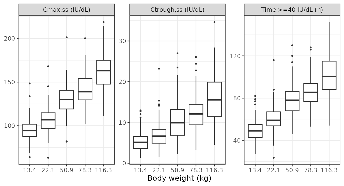
Replicates Figure 2 of Wong 2025: steady-state trough, peak and time above 40 IU/dL across body weight for 50 IU/kg once weekly.
Bleed RTTE validation
Probability of being bleed-free for one year (Table 2)
Table 2 reports the probability of being free of treated bleeds over
the first year of 50 IU/kg once-weekly prophylaxis for a typical patient
in each age group: 78.3 kg for adults/adolescents, 32.8 kg for children
6 to <12 years and 18 kg for children <6 years. For a typical
patient (all random effects zero) this is sur at one year,
a deterministic quantity.
make_rtte_events <- function(wt, id, regimen_ondemand = 0) {
  ev <- rxode2::et(amt = 50 * wt, ii = 168, addl = 52, cmt = "central") |>
    rxode2::et(seq(0, 8760, by = 4), cmt = "central") |>
    as.data.frame()
  ev$id <- id
  ev$WT <- wt
  ev$RACE_ASIAN <- 0
  ev$REGIMEN_ONDEMAND <- regimen_ondemand
  ev
}

typ_rtte <- bind_rows(
  rxode2::rxSolve(rxode2::zeroRe(mod_ad), make_rtte_events(78.3, 1), returnType = "data.frame") |>
    mutate(group = "Adults/adolescents, 78.3 kg"),
  rxode2::rxSolve(rxode2::zeroRe(mod_pe), make_rtte_events(32.8, 1), returnType = "data.frame") |>
    mutate(group = "Children 6 to <12 years, 32.8 kg"),
  rxode2::rxSolve(rxode2::zeroRe(mod_pe), make_rtte_events(18, 1), returnType = "data.frame") |>
    mutate(group = "Children <6 years, 18 kg")
)
#> ℹ omega/sigma items treated as zero: 'etalcl', 'etalvc', 'etalhaz'
#> ℹ omega/sigma items treated as zero: 'etalcl', 'etalvc', 'etalhaz'
#> ℹ omega/sigma items treated as zero: 'etalcl', 'etalvc', 'etalhaz'

tab2 <- typ_rtte |>
  dplyr::filter(time == 8760) |>
  transmute(group, sim = 100 * sur) |>
  mutate(pub = c(71, 74, 72), pub_ci = c("50-83", "59-87", "56-86"))

tab2 |>
  mutate(sim = round(sim, 1)) |>
  dplyr::rename(
    "Typical patient" = group,
    "Bleed-free at 1 year, model (%)" = sim,
    "Table 2 (%)" = pub,
    "Table 2 95% CI" = pub_ci
  ) |>
knitr::kable(caption = "Typical-patient probability of no treated bleed in the first year.")| Typical patient | Bleed-free at 1 year, model (%) | Table 2 (%) | Table 2 95% CI |
|---|---|---|---|
| Adults/adolescents, 78.3 kg | 70.2 | 71 | 50-83 |
| Children 6 to <12 years, 32.8 kg | 74.0 | 74 | 59-87 |
| Children <6 years, 18 kg | 71.7 | 72 | 56-86 |
stopifnot(
  # Deterministic typical-value solve: lambda, gamma, beta, alpha and the
  # embedded PK all enter this one number.
  all(abs(tab2$sim - tab2$pub) < 2)
)
ggplot(typ_rtte, aes(time / 24 / 7, sur, colour = group)) +
  geom_line() +
  labs(x = "Weeks since first dose", y = "Probability of no treated bleed", colour = NULL) +
  theme_bw() +
  theme(legend.position = "bottom")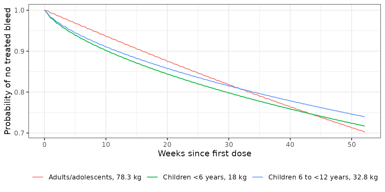
Typical-patient survivor functions underlying Table 2 of Wong 2025.
Hazard over a steady-state dosing week
The FVIII effect makes the bleed hazard rise through each dosing interval as FVIII activity falls. The plot shows one steady-state week (week 50) for the three typical patients.
typ_rtte |>
  dplyr::filter(time >= 168 * 50, time <= 168 * 51) |>
  mutate(day = (time - 168 * 50) / 24) |>
  ggplot(aes(day, hazard * 24 * 365.25, colour = group)) +
  geom_line() +
  labs(x = "Days after the weekly dose", y = "Hazard (bleeds per year)", colour = NULL) +
  theme_bw() +
  theme(legend.position = "bottom")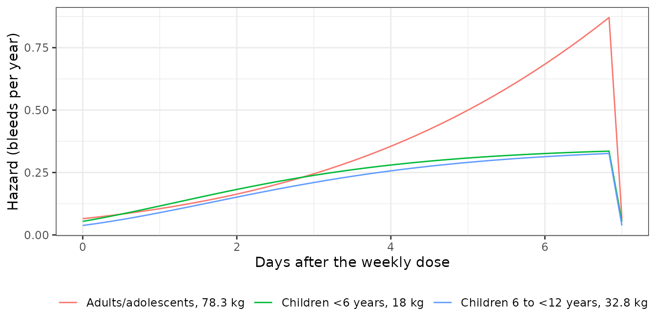
Annualized bleed rate in virtual populations (Table 2)
Table 2 also reports the mean annualized bleed rate (ABR) in virtual populations with IIV in both PK and hazard: adults/adolescents of mean (SD) body weight 79.3 (19.8) kg, children 6 to <12 years of 35.5 (13.6) kg and children <6 years of 16.2 (4.7) kg. With the hazard evaluated on time since the first dose, the number of bleeds in a year for patient is Poisson with mean , where is the cumulative hazard with the hazard random effect at zero. So the expected ABR and the probability of no bleeds can be computed exactly over the hazard random effect, leaving only the PK random effects and body weight to sample (200 virtual patients per group).
n_abr <- 200
draw_wt <- function(n, mean, sd, lo, hi) {
  out <- numeric(0)
  while (length(out) < n) {
    w <- rnorm(n, mean, sd)
    out <- c(out, w[w >= lo & w <= hi])
  }
  out[seq_len(n)]
}
groups <- data.frame(
  group = c("Adults/adolescents", "Children 6 to <12 years", "Children <6 years"),
  wt_mean = c(79.3, 35.5, 16.2), wt_sd = c(19.8, 13.6, 4.7),
  wt_lo = c(33.9, 17.2, 11.4), wt_hi = c(133, 66.5, 25.7),
  omega2 = c(0.8327, 1.4951, 1.4951),
  abr_pub = c(0.71, 0.70, 0.76)
)
omega_pk <- matrix(c(0.0354, 0.0148, 0.0148, 0.0209), 2)

cum_haz <- function(g) {
  wt <- draw_wt(n_abr, groups$wt_mean[g], groups$wt_sd[g], groups$wt_lo[g], groups$wt_hi[g])
  eta <- rxode2::rxRmvn(n_abr, c(0, 0), omega_pk)
  ev <- bind_rows(lapply(seq_len(n_abr), function(i) {
    e <- make_rtte_events(wt[i], i)
    e[e$evid != 0 | e$time %in% c(0, 8760), ]
  }))
  prm <- data.frame(id = seq_len(n_abr), lcl = log(0.433) + eta[, 1], lvc = log(30.2) + eta[, 2])
  m <- if (g == 1) mod_ad else mod_pe
  s <- rxode2::rxSolve(rxode2::zeroRe(m), ev, params = prm, returnType = "data.frame") |>
    suppressWarnings()
  s$cumhaz[s$time == 8760]
}

# Gauss-type integration over the hazard random effect on a fixed grid.
z <- seq(-8, 8, by = 0.01)
wz <- dnorm(z) * 0.01
abr <- bind_rows(lapply(seq_len(nrow(groups)), function(g) {
  H <- cum_haz(g)
  w <- sqrt(groups$omega2[g])
  data.frame(
    group = groups$group[g],
    abr_sim = mean(H) * exp(groups$omega2[g] / 2),
    p0_sim = 100 * mean(vapply(H, function(h) sum(exp(-h * exp(w * z)) * wz), numeric(1))),
    abr_pub = groups$abr_pub[g]
  )
}))
#> ℹ omega/sigma items treated as zero: 'etalcl', 'etalvc', 'etalhaz'
#> ℹ omega/sigma items treated as zero: 'etalcl', 'etalvc', 'etalhaz'
#> ℹ omega/sigma items treated as zero: 'etalcl', 'etalvc', 'etalhaz'
# The same cohort under the alternative reading omega^2 = CV^2.
abr$abr_cv2 <- abr$abr_sim * exp((c(1.14, 1.86, 1.86)^2 - groups$omega2) / 2)

abr |>
  mutate(p0_pub = c("64", "not reported", "not reported")) |>
  mutate(across(c(abr_sim, abr_cv2, p0_sim), \(x) signif(x, 3))) |>
  select(group, abr_sim, abr_cv2, abr_pub, p0_sim, p0_pub) |>
  dplyr::rename(
    "Virtual population" = group,
    "Mean ABR, model" = abr_sim,
    "Mean ABR if omega^2 = CV^2" = abr_cv2,
    "Mean ABR, Table 2" = abr_pub,
    "No bleeds in 1 year, model (%)" = p0_sim,
    "No bleeds, Results (%)" = p0_pub
  ) |>
knitr::kable(caption = "Virtual-population ABR and proportion without bleeds, 50 IU/kg once weekly.")| Virtual population | Mean ABR, model | Mean ABR if omega^2 = CV^2 | Mean ABR, Table 2 | No bleeds in 1 year, model (%) | No bleeds, Results (%) |
|---|---|---|---|---|---|
| Adults/adolescents | 0.577 | 0.728 | 0.71 | 64.3 | 64 |
| Children 6 to <12 years | 0.619 | 1.650 | 0.70 | 66.9 | not reported |
| Children <6 years | 0.708 | 1.890 | 0.76 | 64.1 | not reported |
stopifnot(
  # The pediatric means are near Table 2; the adult/adolescent mean is
  # lower (parameter uncertainty, next chunk), but the proportion without
  # bleeds agrees with the published 64%.
  all(abs(abr$abr_sim[2:3] / abr$abr_pub[2:3] - 1) < 0.25),
  # The alternative omega^2 = CV^2 reading overshoots the pediatric means
  # more than two-fold.
  all(abr$abr_cv2[2:3] / abr$abr_pub[2:3] > 2),
  abs(abr$p0_sim[1] - 64) < 6
)
With the point estimates, the pediatric ABRs are about 10% below Table 2 and the adult/adolescent ABR about 20% below, while the proportion of adults with no bleeds (64% published) agrees. The paper’s simulations incorporated parameter uncertainty (Methods, Simulations). Because the hazard is convex in its parameters, uncertainty raises the mean ABR: for adults mainly through (RSE 14.5%) and (RSE 11.2%), for children through (RSE 58.2%). The next chunk redraws the four structural RTTE parameters from their RSEs (log-normal for , normal for the others; an approximation, since the paper gives no covariance matrix) and recomputes the mean ABR on the same virtual patients’ FVIII profiles. The hazard expression is the model’s, evaluated in R so that 200 parameter draws need only one PK solve.
rtte_par <- list(
  list(lam = 0.00247, gam = 1.02, bet = -1.73, alp = 0.247, rse = c(0.362, 0.0631, 0.145, 0.112)),
  list(lam = 0.0000429, gam = 0.694, bet = -0.00535, alp = 1.27, rse = c(0.582, 0.145, 0.0155, 0.0437))
)
t_grid <- seq(0, 8760, by = 2)
abr_unc <- bind_rows(lapply(seq_len(nrow(groups)), function(g) {
  wt <- draw_wt(n_abr, groups$wt_mean[g], groups$wt_sd[g], groups$wt_lo[g], groups$wt_hi[g])
  ev <- bind_rows(lapply(seq_len(n_abr), function(i) {
    e <- rxode2::et(amt = 50 * wt[i], ii = 168, addl = 52, cmt = "central") |>
      rxode2::et(t_grid, cmt = "central") |>
      as.data.frame()
    e$id <- i
    e$WT <- wt[i]
    e$RACE_ASIAN <- 0
    e
  }))
  conc <- rxode2::rxSolve(mod_pk, ev, returnType = "data.frame") |>
    select(id, time, Cc)
  cmat <- matrix(pmax(conc$Cc, 0), nrow = length(t_grid))
  p <- rtte_par[[if (g == 1) 1 else 2]]
  draws <- vapply(seq_len(200), function(k) {
    lam <- p$lam * exp(rnorm(1, 0, p$rse[1]))
    gam <- p$gam * (1 + rnorm(1, 0, p$rse[2]))
    bet <- p$bet * (1 + rnorm(1, 0, p$rse[3]))
    alp <- p$alp * (1 + rnorm(1, 0, p$rse[4]))
    h <- lam * gam * (lam * pmax(t_grid, 1e-4))^(gam - 1) * exp(bet * cmat^alp)
    H <- colSums((h[-1, , drop = FALSE] + h[-nrow(h), , drop = FALSE]) / 2 * diff(t_grid))
    mean(H) * exp(groups$omega2[g] / 2)
  }, numeric(1))
  data.frame(group = groups$group[g], abr_unc = mean(draws), abr_pub = groups$abr_pub[g])
}))

abr_unc |>
  left_join(select(abr, group, abr_sim), by = "group") |>
  mutate(across(c(abr_sim, abr_unc), \(x) signif(x, 3))) |>
  select(group, abr_sim, abr_unc, abr_pub) |>
  dplyr::rename(
    "Virtual population" = group,
    "Mean ABR, point estimates" = abr_sim,
    "Mean ABR, with parameter uncertainty" = abr_unc,
    "Mean ABR, Table 2" = abr_pub
  ) |>
knitr::kable(caption = "Effect of RTTE parameter uncertainty on the simulated mean ABR.")| Virtual population | Mean ABR, point estimates | Mean ABR, with parameter uncertainty | Mean ABR, Table 2 |
|---|---|---|---|
| Adults/adolescents | 0.577 | 0.754 | 0.71 |
| Children 6 to <12 years | 0.619 | 0.673 | 0.70 |
| Children <6 years | 0.708 | 0.829 | 0.76 |
stopifnot(
  # With parameter uncertainty every group's mean ABR moves to the
  # published value. The band allows for the 200-patient PK sample and the
  # 200 parameter draws.
  all(abs(abr_unc$abr_unc / abr_unc$abr_pub - 1) < 0.2)
)
With parameter uncertainty all three mean ABRs agree with Table 2 to within 20%. The packaged models carry the point estimates only.
Assumptions and deviations
- Hazard IIV scale. Table S6 reports the IIV on the base hazard as 114 and 186 CV%. These were converted to log-scale variances with , giving 0.8327 and 1.4951, the same log-normal convention that reproduces the %CV column of the paper’s own PopPK table (Table S4). The virtual-population ABRs confirm this reading: under it, and with parameter uncertainty, all three groups match Table 2, whereas (3.46 for children) gives pediatric ABRs more than twice the published 0.70-0.76.
- Where the random effect enters. The printed hazard equation multiplies the whole hazard by ; the models follow it rather than placing on inside .
- On-demand effect on . The Results state that “the hazard () for a bleeding episode was ~9-fold higher for on-demand treatment”, so the 2.21 log-fold effect is applied to . Because enters the Weibull hazard as , the whole-hazard ratio is rather than ; applying the effect to the hazard instead would differ by less than 5%.
-
On-demand simulation. Patients treated on demand
receive doses only to treat bleeds, so simulating
REGIMEN_ONDEMAND = 1meaningfully needs an event table with bleed-triggered doses. With no doses at all, FVIII activity is zero and the model predicts a far higher bleed rate than was observed on demand in XTEND-1. - Time origin of the Weibull hazard. The hazard is evaluated on time since the start of efanesoctocog alfa treatment. The paper does not say whether the time variable was reset after each bleed. It makes no difference for the first-bleed probabilities in Table 2, and little for adults, whose is close to a constant hazard. The typical-patient probabilities reproduce Table 2 when the simulation starts at the first dose.
- Hazard at time zero. With (children) the base hazard is infinite at . The models floor at h, which changes the cumulative hazard by less than .
- PopPK IIV and covariance. Table S4 lists log-scale variances of 0.0354 and 0.0209 (their %CV values follow from ) and a ‘Corr-CL-V’ of 0.0148. The latter is used as the covariance (correlation 0.544): read as a correlation coefficient it would imply essentially no correlation, which is inconsistent with its 21.6% RSE and with the base model being built with correlation between CL and V.
- Residual error. The combined additive (0.837 IU/dL) and proportional (0.182) error is encoded with nlmixr2’s default combined form; the paper does not say how the two terms were combined. The 0.182 is read as an SD, since a variance would imply a 43% proportional error against an assay precision within 20%. Samples below the 1 IU/dL LLOQ (about 3%) are not modelled.
-
RTTE output. The source fits the RTTE likelihood
directly. The packaged RTTE files expose the cumulative hazard, the
survivor function
surand thehazard, and attach a placeholder additive error (SD 0.001) tosurso the model can be used for simulation; this error is not from the source. The PK residual error is not carried into the RTTE files. -
Covariate column for treatment strategy. The
on-demand vs prophylaxis contrast uses the
REGIMEN_ONDEMANDcolumn (1 = on demand, 0 = scheduled prophylaxis), registered for this model. For XTEND-1 Arm B it is time-varying: 1 for the first 26 weeks and 0 after the switch to prophylaxis. - Virtual cohorts. All virtual patients are non-Asian. Body weights for the ABR populations are drawn from normal distributions with the published means and SDs, redrawn to stay within the observed weight range of each RTTE dataset (Tables S5 and S7).
- Body weight is time-varying in the source PopPK analysis; the simulations here hold it constant within each patient.