Liraglutide (Carlsson Petri 2015) • nlmixr2lib

Model and source

Citation: Carlsson Petri KC, Jacobsen LV, Klein DJ. Comparable liraglutide pharmacokinetics in pediatric and adult populations with type 2 diabetes: a population pharmacokinetic analysis. Clin Pharmacokinet. 2015;54(6):663-670. doi:10.1007/s40262-014-0229-z
Description: Liraglutide population PK model in pediatric (10-17 y) and adult subjects with type 2 diabetes (Carlsson Petri 2015 pooled three-trial analysis)
Article: https://doi.org/10.1007/s40262-014-0229-z
Supplement (Online Resource, Springer ESM): https://static-content.springer.com/esm/art%3A10.1007%2Fs40262-014-0229-z/MediaObjects/40262_2014_229_MOESM1_ESM.pdf

The main article does not print any parameter estimates. Every structural parameter, covariate coefficient, between-subject variance, and residual-error term in this model comes from Table 1 of the Online Resource (ESM), “Parameter estimates of the full and base models”. The model file encodes the full model column throughout; the base-model column is quoted in the in-file comments for context only.

Population

The model was fitted to pooled data from three trials in subjects with type 2 diabetes (T2D), 57 subjects in total (main article Table 1):

Trial 1 (NCT00943501) – 13 pediatric subjects, 10-17 years, 62 % female, median body weight 106 kg (range 57-214). Weekly dose escalation 0.3 -> 0.6 -> 0.9 -> 1.2 -> 1.8 mg once daily subcutaneously, with PK profiles taken at the 0.3, 0.6, 1.2 and 1.8 mg levels (four profiles per subject).
Trial 2 (NCT00993304) – 12 adults, 54-73 years, 50 % female, median body weight 83 kg (range 72-104). Steady-state 1.8 mg once daily.
Trial 3 (NCT00873223) – 32 adults, 33-68 years, 28 % female, median body weight 96 kg (range 58-140). Steady-state 1.8 mg once daily.

Subjects with impaired renal function were excluded from all three trials. The pediatric cohort’s median body weight exceeds both adult cohorts, driven partly by a single 214 kg subject.

The same information is available programmatically via readModelDb("CarlssonPetri_2015_liraglutide")()$population.

Model structure

One compartment, first-order absorption, first-order elimination, parameterised as ka, CL/F and V/F with bioavailability fixed at 1. Covariate effects act on CL/F only; V/F carries none. ESM Table 1 footnote ** gives the clearance model as

CL_i/F = (CL/F) * (BWT / 90 kg)^CovCLBWT
         * exp(CovCLGen if male) * exp(CovCLPaed if paediatric) * exp(eta_i)

with female and adult as the reference categories, so the reference subject is an adult female weighing 90 kg.

Source trace

Equation / parameter	Value	Source location
`lka` (ka)	0.0657 1/h (RSE 6 %)	ESM Table 1, row `KA`, full-model column
`lcl` (CL/F)	1.06 L/h (RSE 10 %)	ESM Table 1, row `CL/F`, full-model column; footnote: reference = adult female, 90 kg
`lvc` (V/F)	15.3 L (RSE 19 %)	ESM Table 1, row `V/F`, full-model column
`lfdepot` (F)	1 (fixed)	ESM Table 1, row `F`
`e_wt_cl`	0.929 (RSE 15 %)	ESM Table 1, row `Cov CL-BWT`
`e_male_cl`	0.365 (RSE 29 %)	ESM Table 1, row `Cov CL-Gen`
`e_child_cl`	0.107 (RSE 91 %)	ESM Table 1, row `Cov CL-AGEgr`
`etalcl`	34 %CV -> omega^2 = 0.1156	ESM Table 1, row `CL/F (dose 1.8 mg)`, “BSV in CL/F”, full model (shrinkage 1 %)
`etalvc`	fixed 0 (not published)	Main article Sect. 2.2 declares BSV on V/F; ESM Table 1 reports no estimate
`propSd`	0.23 (23 %CV)	ESM Table 1, row `Sigma`, residual error (proportional), shrinkage 7 %
CL/F covariate equation	n/a	ESM Table 1, footnote `**`
Reference weight 90 kg	n/a	Main article Sect. 2.2 and the ESM Table 1 equation
Dose units (nmol)	n/a	Main article Sect. 2.2: `AUC24 = dose (in nmol) / (CL/F)`

Scale checks performed while transcribing

Two reporting scales in ESM Table 1 are ambiguous on their face and were settled against numbers printed independently in the main article:

The %CV columns are on the NONMEM variance scale (omega^2 = (CV/100)^2), not the exact log-normal scale (omega^2 = log(1 + CV^2)). Results states that “the inclusion of covariates reduced between-subject variability in CL/F by 50 %” relative to the base model. With BSV 34 %CV (full) and 48 %CV (base):

variance_scale <- 1 - 0.34^2 / 0.48^2
lognormal_scale <- 1 - log(1 + 0.34^2) / log(1 + 0.48^2)
cv_scale <- 1 - 0.34 / 0.48

data.frame(
  Reading = c("variance: omega^2 = CV^2",
              "exact log-normal: omega^2 = log(1 + CV^2)",
              "CV scale"),
  `Implied reduction` = sprintf("%.1f %%", 100 * c(variance_scale, lognormal_scale, cv_scale)),
  check.names = FALSE
) |>
  knitr::kable(caption = "Which omega scale reproduces the article's printed 50 % BSV reduction.")

Which omega scale reproduces the article’s printed 50 % BSV reduction.
Reading	Implied reduction
variance: omega^2 = CV^2	49.8 %
exact log-normal: omega^2 = log(1 + CV^2)	47.2 %
CV scale	29.2 %


# The variance reading is the only one that rounds to the printed 50 %.
stopifnot(abs(100 * variance_scale - 50) < 0.5)

The KA unit is a typographical error. ESM Table 1 labels the absorption rate constant “L/h”; a first-order rate constant is 1/h. The magnitude confirms it: log(2)/0.0657 = 10.6 h absorption half-life, consistent with liraglutide’s 8-12 h tmax and with the sibling Overgaard_2016_liraglutide model’s 0.0806 1/h.

Virtual cohort

Original subject-level data are not public. The cohorts below reproduce each trial’s published sex balance and body-weight median/range using a truncated log-normal weight distribution. 200 subjects per arm.

# set.seed() seeds R's RNG (used for the covariate draws below). It does NOT
# seed rxode2's simulation RNG, whose streams are partitioned per solver
# thread -- so the eta draws differ between a 2-core CI runner and a 16-thread
# workstation. Every assertion below is written to hold for any cohort this
# model can produce (centre and robust quantiles), or is deterministic
# (zeroRe(), closed-form identities).
set.seed(20150121)

MW_LIRAGLUTIDE <- 3751.2 # g/mol; used to convert the clinical mg doses to nmol
mg_to_nmol <- function(mg) mg * 1e6 / MW_LIRAGLUTIDE

TAU <- 24        # dosing interval (h)
N_DOSES <- 12    # 12 once-daily doses; the last lands at t = 264 h
SS_START <- (N_DOSES - 1) * TAU
SS_END <- SS_START + TAU

# 264 h is ~25 half-lives at the model's slower disposition rate constant
# (ka = 0.0657 1/h is slower than kel = 1.06/15.3 = 0.0693 1/h, so absorption
# is rate-limiting and governs the approach to steady state).
stopifnot(SS_START / (log(2) / 0.0657) > 20)

draw_weights <- function(n, median_wt, lo, hi, sdlog) {
  wt <- stats::rlnorm(n, meanlog = log(median_wt), sdlog = sdlog)
  pmin(pmax(wt, lo), hi)
}

make_arm <- function(n, arm, dose_mg, median_wt, wt_lo, wt_hi, sdlog,
                     pct_female, child, id_offset) {
  subj <- tibble(
    id = id_offset + seq_len(n),
    arm = arm,
    WT = draw_weights(n, median_wt, wt_lo, wt_hi, sdlog),
    SEXF = as.numeric(seq_len(n) <= round(n * pct_female / 100)),
    CHILD = as.numeric(child)
  )
  doses <- subj |>
    mutate(time = 0, amt = mg_to_nmol(dose_mg), evid = 1L,
           ii = TAU, addl = N_DOSES - 1L, cmt = "depot")
  obs <- subj |>
    tidyr::crossing(time = seq(SS_START, SS_END, by = 0.25)) |>
    mutate(amt = 0, evid = 0L, ii = 0, addl = 0L, cmt = "central")
  bind_rows(doses, obs) |> arrange(id, time, desc(evid))
}

events <- bind_rows(
  # Trial 1 (pediatric) at each dose level with a PK profile. Each arm draws
  # its own 200 subjects from the same Trial 1 covariate distribution, so the
  # four arms are statistically exchangeable but not subject-matched.
  make_arm(200, "0.3 mg", 0.3, 106, 57, 214, 0.30, 62, 1,    0L),
  make_arm(200, "0.6 mg", 0.6, 106, 57, 214, 0.30, 62, 1,  200L),
  make_arm(200, "1.2 mg", 1.2, 106, 57, 214, 0.30, 62, 1,  400L),
  make_arm(200, "Trial 1 (pediatric)", 1.8, 106, 57, 214, 0.30, 62, 1,  600L),
  # Adult comparator trials, 1.8 mg only.
  make_arm(200, "Trial 2 (adult)", 1.8,  83, 72, 104, 0.10, 50, 0,  800L),
  make_arm(200, "Trial 3 (adult)", 1.8,  96, 58, 140, 0.21, 28, 0, 1000L)
)

stopifnot(
  !anyDuplicated(events[events$evid == 0L, c("id", "time")]),
  all(table(unique(events[, c("id", "arm")])$arm) == 200)
)

Reproduced cohort characteristics against the published Table 1:

events |>
  distinct(id, arm, WT, SEXF) |>
  group_by(arm) |>
  summarise(
    n = n(),
    `Median WT (kg)` = round(median(WT), 1),
    `WT range (kg)` = sprintf("%.0f-%.0f", min(WT), max(WT)),
    `Female (%)` = round(100 * mean(SEXF)),
    .groups = "drop"
  ) |>
  knitr::kable(caption = "Simulated cohort covariates. The four pediatric dose arms share the Trial 1 distribution.")

Simulated cohort covariates. The four pediatric dose arms share the Trial 1 distribution.
arm	n	Median WT (kg)	WT range (kg)	Female (%)
0.3 mg	200	102.7	57-214	62
0.6 mg	200	106.3	57-214	62
1.2 mg	200	106.3	57-214	62
Trial 1 (pediatric)	200	107.5	57-214	62
Trial 2 (adult)	200	82.6	72-104	50
Trial 3 (adult)	200	97.7	58-140	28

Simulation

mod <- readModelDb("CarlssonPetri_2015_liraglutide")

sim <- rxode2::rxSolve(
  mod,
  events = as.data.frame(events),
  keep = c("arm", "WT", "SEXF", "CHILD"),
  returnType = "data.frame"
)
#> ℹ parameter labels from comments will be replaced by 'label()'
#> ℹ omega/sigma items treated as zero: 'etalvc'

# A large proportional residual can push simulated concentrations negative,
# which would make the NCA log-linear steps return NaN. Guard explicitly.
stopifnot(!anyNA(sim$Cc), all(sim$Cc > 0))

Replicate published figures

Figure 1 – pediatric concentration-time profiles by dose level

# Replicates Figure 1 of Carlsson Petri 2015: observed and model-derived
# liraglutide concentration profiles in the pediatric population by dose
# level. The published figure overlays observed geometric means (with 95 %
# CI bars) on geometric means of the individual post-hoc profiles; only the
# model-derived side can be reproduced here.
geomean <- function(x) exp(mean(log(x)))

sim |>
  # rxSolve() returns only the observation grid and does not carry `evid`
  # through, so no evid filter is needed (or possible) on `sim`.
  filter(arm %in% c("0.3 mg", "0.6 mg", "1.2 mg", "Trial 1 (pediatric)")) |>
  mutate(
    dose_level = factor(
      ifelse(arm == "Trial 1 (pediatric)", "1.8 mg", arm),
      levels = c("0.3 mg", "0.6 mg", "1.2 mg", "1.8 mg")
    ),
    tad = time - SS_START
  ) |>
  group_by(dose_level, tad) |>
  summarise(
    gm = geomean(Cc),
    lo = quantile(Cc, 0.05),
    hi = quantile(Cc, 0.95),
    .groups = "drop"
  ) |>
  ggplot(aes(tad, gm)) +
  geom_ribbon(aes(ymin = lo, ymax = hi), alpha = 0.2) +
  geom_line(linewidth = 0.8) +
  facet_wrap(~dose_level) +
  labs(
    x = "Time since last dose (h)", y = "Liraglutide concentration (nM)",
    title = "Figure 1 -- pediatric steady-state profiles by dose level",
    caption = "Replicates the model-derived side of Figure 1 of Carlsson Petri 2015.\nLine = geometric mean; band = 5th-95th percentile."
  )

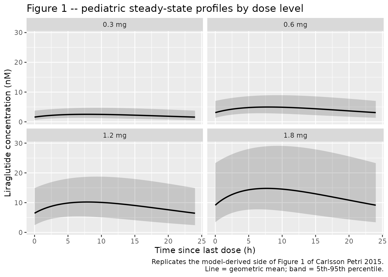
Figure 3 – covariate effects on AUC24 (deterministic gate)

This is the strongest available check: the article prints four covariate effect sizes in Results, and every one of them is a deterministic typical-value ratio that the packaged model must reproduce exactly. The simulation below uses zeroRe(), so there is no cohort randomness in this comparison.

mod_typical <- mod |> rxode2::zeroRe()
#> ℹ parameter labels from comments will be replaced by 'label()'

typical_scenarios <- tibble::tribble(
  ~scenario,               ~WT, ~SEXF, ~CHILD,
  "Reference (adult female, 90 kg)", 90,     1,      0,
  "Body weight 53 kg",              53,     1,      0,
  "Body weight 216 kg",            216,     1,      0,
  "Male",                           90,     0,      0,
  "Pediatric",                      90,     1,      1
) |>
  mutate(id = row_number())

typical_events <- bind_rows(
  typical_scenarios |>
    mutate(time = 0, amt = mg_to_nmol(1.8), evid = 1L,
           ii = TAU, addl = N_DOSES - 1L, cmt = "depot"),
  typical_scenarios |>
    tidyr::crossing(time = seq(SS_START, SS_END, by = 0.05)) |>
    mutate(amt = 0, evid = 0L, ii = 0, addl = 0L, cmt = "central")
) |>
  arrange(id, time, desc(evid))

sim_typical <- rxode2::rxSolve(
  mod_typical, events = as.data.frame(typical_events),
  keep = c("scenario"), returnType = "data.frame"
)
#> ℹ omega/sigma items treated as zero: 'etalcl', 'etalvc'
#> Warning: multi-subject simulation without without 'omega'

# AUC24 at steady state, by the trapezoidal rule on a 0.05 h grid.
auc24_typical <- sim_typical |>
  group_by(scenario) |>
  summarise(
    auc24 = sum(diff(time) * (head(Cc, -1) + tail(Cc, -1)) / 2),
    cl = unique(cl),
    .groups = "drop"
  )

ref_auc <- auc24_typical$auc24[auc24_typical$scenario == "Reference (adult female, 90 kg)"]
stopifnot(length(ref_auc) == 1L)

forest <- auc24_typical |>
  filter(scenario != "Reference (adult female, 90 kg)") |>
  mutate(ratio = auc24 / ref_auc) |>
  left_join(
    tibble::tribble(
      ~scenario,            ~published_ratio, ~published_text,
      "Body weight 53 kg",  1.64,             "64 % higher at the lowest observed body weight (53 kg)",
      "Body weight 216 kg", 0.44,             "56 % lower at the highest observed body weight (216 kg)",
      "Male",               0.69,             "31 % lower drug exposure compared with the reference female subject",
      "Pediatric",          0.90,             "10 % decrease in AUC24 compared with an adult subject of the same weight and gender"
    ),
    by = "scenario"
  )

stopifnot(nrow(forest) == 4L, !anyNA(forest$published_ratio))

forest |>
  mutate(
    Simulated = round(ratio, 3),
    Published = published_ratio,
    `% diff` = round(100 * (ratio - published_ratio) / published_ratio, 2)
  ) |>
  select(scenario, Simulated, Published, `% diff`, published_text) |>
  rename(
    "Covariate scenario" = scenario,
    "Simulated AUC24 ratio" = Simulated,
    "Published AUC24 ratio" = Published,
    "Source sentence (Results)" = published_text
  ) |>
  knitr::kable(caption = "Figure 3 covariate effects: deterministic typical-value AUC24 ratios versus the values printed in Results.")

Figure 3 covariate effects: deterministic typical-value AUC24 ratios versus the values printed in Results.
Covariate scenario	Simulated AUC24 ratio	Published AUC24 ratio	% diff	Source sentence (Results)
Body weight 216 kg	0.443	0.44	0.77	56 % lower at the highest observed body weight (216 kg)
Body weight 53 kg	1.635	1.64	-0.28	64 % higher at the lowest observed body weight (53 kg)
Male	0.694	0.69	0.61	31 % lower drug exposure compared with the reference female subject
Pediatric	0.899	0.90	-0.16	10 % decrease in AUC24 compared with an adult subject of the same weight and gender


# Deterministic on both sides (zeroRe(), same solver, closed-form covariate
# algebra), so the only slack needed is the article's own 2-significant-figure
# rounding of each printed effect. 1.5 % covers that and nothing more.
stopifnot(all(abs(forest$ratio - forest$published_ratio) / forest$published_ratio < 0.015))

forest |>
  mutate(scenario = factor(scenario, levels = rev(scenario))) |>
  ggplot(aes(ratio, scenario)) +
  geom_vline(xintercept = 1, linewidth = 0.6) +
  geom_vline(xintercept = c(0.8, 1.25), linetype = "dashed") +
  geom_point(size = 3) +
  geom_point(aes(x = published_ratio), shape = 4, size = 3, colour = "red") +
  scale_x_log10() +
  labs(
    x = "AUC24 ratio vs reference (90 kg adult female)", y = NULL,
    title = "Figure 3 -- covariate effects on AUC24",
    caption = "Replicates Figure 3 of Carlsson Petri 2015. Dots = packaged model; red crosses = published values.\nDashed lines delineate the 0.80-1.25 bioequivalence acceptance interval."
  )

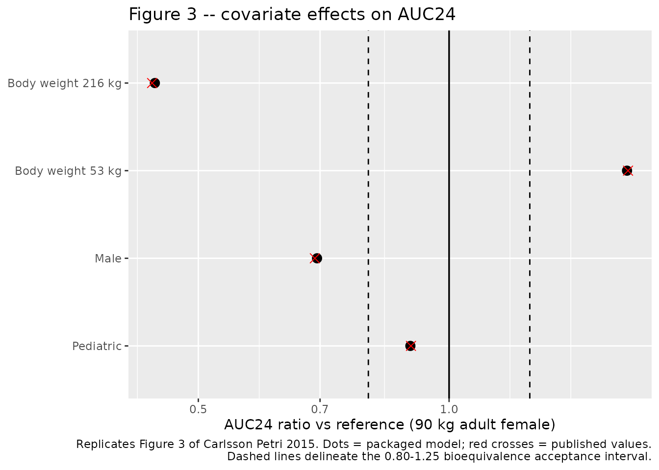
Figure 4b – pediatric versus adult typical profiles at matched covariates

# Replicates Figure 4b of Carlsson Petri 2015: model-derived typical
# steady-state profiles for pediatric and adult subjects on 1.8 mg, with
# body weight and sex matched (90 kg, 50 % female) to remove confounding.
fig4b_scenarios <- tidyr::crossing(
  CHILD = c(0, 1),
  SEXF = c(0, 1)
) |>
  mutate(WT = 90, id = row_number(),
         population = ifelse(CHILD == 1, "Pediatric", "Adult"))

fig4b_events <- bind_rows(
  fig4b_scenarios |>
    mutate(time = 0, amt = mg_to_nmol(1.8), evid = 1L,
           ii = TAU, addl = N_DOSES - 1L, cmt = "depot"),
  fig4b_scenarios |>
    tidyr::crossing(time = seq(SS_START, SS_END, by = 0.25)) |>
    mutate(amt = 0, evid = 0L, ii = 0, addl = 0L, cmt = "central")
) |>
  arrange(id, time, desc(evid))

sim_4b <- rxode2::rxSolve(
  mod_typical, events = as.data.frame(fig4b_events),
  keep = c("population", "SEXF"), returnType = "data.frame"
)
#> ℹ omega/sigma items treated as zero: 'etalcl', 'etalvc'
#> Warning: multi-subject simulation without without 'omega'

# A 50 % female composition is represented by the geometric mean of the
# male and female typical profiles at each time point.
sim_4b |>
  mutate(tad = time - SS_START) |>
  group_by(population, tad) |>
  summarise(Cc = geomean(Cc), .groups = "drop") |>
  ggplot(aes(tad, Cc, colour = population, linetype = population)) +
  geom_line(linewidth = 0.9) +
  labs(
    x = "Time since last dose (h)", y = "Liraglutide concentration (nM)",
    colour = NULL, linetype = NULL,
    title = "Figure 4b -- typical steady-state profiles, 1.8 mg, 90 kg, 50 % female",
    caption = "Replicates Figure 4b of Carlsson Petri 2015."
  )

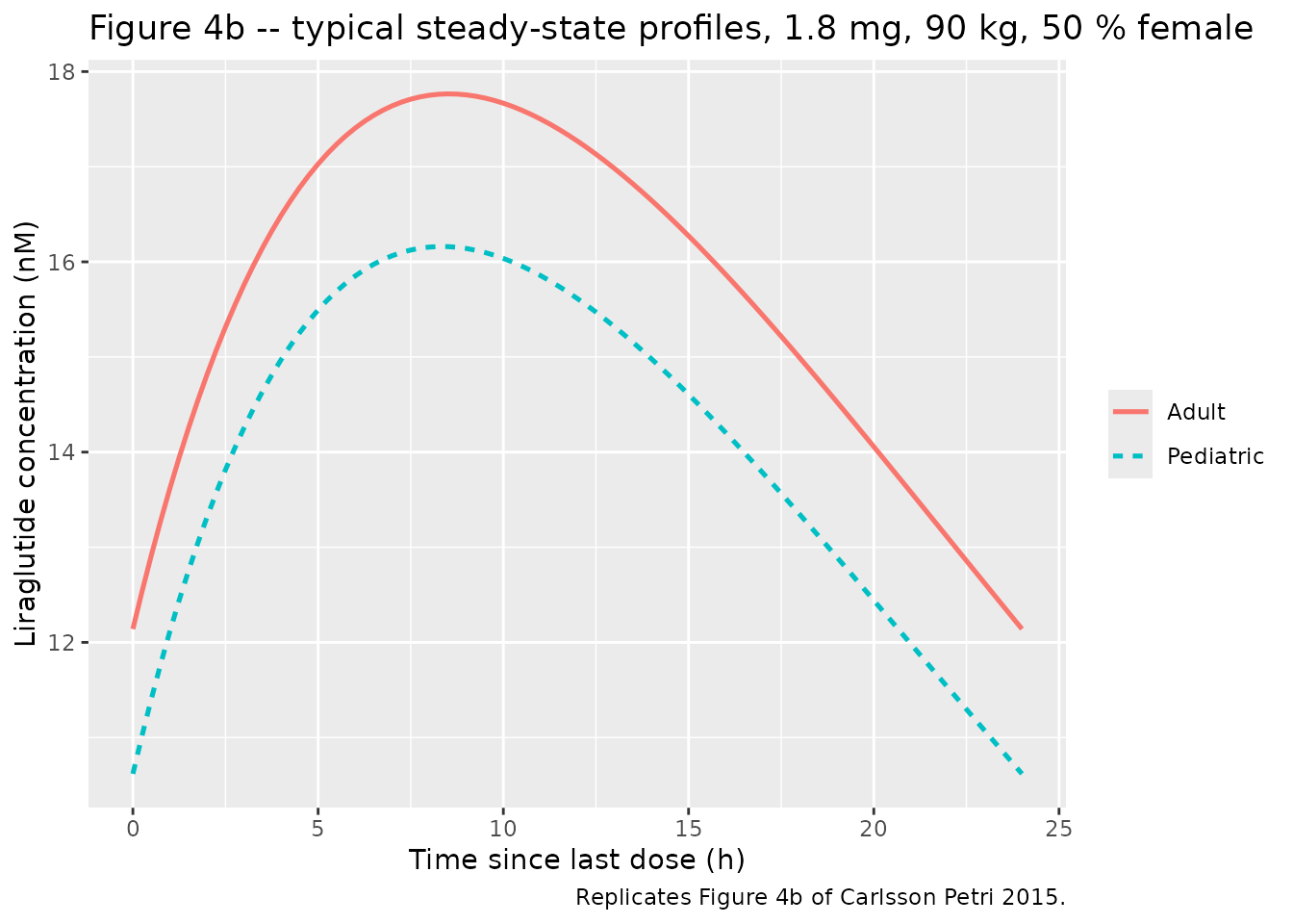
The two profiles sit 10 % apart at every time point – the whole of the age-category effect – which is the paper’s basis for concluding that “liraglutide concentration-time profiles for pediatric and adult subjects treated with the 1.8 mg dose appeared very similar”.

PKNCA validation

sim_nca <- sim |>
  filter(!is.na(Cc)) |>
  select(id, time, Cc, arm)

conc_obj <- PKNCA::PKNCAconc(
  as.data.frame(sim_nca), Cc ~ time | arm + id,
  concu = "nmol/L", timeu = "h"
)

dose_df <- events |>
  filter(evid == 1L) |>
  # PKNCA anchors the steady-state interval on the dose at its start; the
  # event table expresses the 12 doses as one row plus addl/ii.
  mutate(time = SS_START) |>
  select(id, time, amt, arm)

dose_obj <- PKNCA::PKNCAdose(
  as.data.frame(dose_df), amt ~ time | arm + id,
  doseu = "nmol"
)

intervals <- data.frame(
  start = SS_START, end = SS_END,
  # `cmin` over a steady-state interval is the trough; PKNCA's `ctrough`
  # is deliberately omitted because it returns NA for this interval shape
  # and would add nothing the paper reports.
  cmax = TRUE, tmax = TRUE, cmin = TRUE,
  auclast = TRUE, cav = TRUE
)

nca_res <- PKNCA::pk.nca(
  PKNCA::PKNCAdata(conc_obj, dose_obj, intervals = intervals)
)

nca_tbl <- as.data.frame(nca_res$result)
stopifnot(nrow(nca_tbl) > 0, !any(is.na(nca_tbl$PPORRES)))

Closed-form gate: AUC0-tau at steady state equals Dose / (CL/F)

With bioavailability fixed at 1 and linear disposition, steady-state AUC over a dosing interval is exactly Dose / (CL/F). Both sides of this comparison use the same drawn parameters, so the only discrepancy is trapezoidal error on the 0.25 h observation grid – a tight bound is correct here.

subject_cl <- sim |>
  distinct(id, arm, cl)

subject_dose <- events |>
  filter(evid == 1L) |>
  select(id, amt)

auc_check <- nca_tbl |>
  filter(PPTESTCD == "auclast") |>
  select(id, arm, auclast = PPORRES) |>
  left_join(subject_cl, by = c("id", "arm")) |>
  left_join(subject_dose, by = "id") |>
  mutate(
    closed_form = amt / cl,
    pct_diff = 100 * (auclast - closed_form) / closed_form
  )

stopifnot(nrow(auc_check) == 1200L, !anyNA(auc_check$pct_diff))

auc_check |>
  summarise(
    `Median % diff` = round(median(pct_diff), 4),
    `Max |% diff|` = round(max(abs(pct_diff)), 4)
  ) |>
  knitr::kable(caption = "Steady-state AUC0-tau from PKNCA versus the closed form Dose / (CL/F), across all 1200 simulated subjects.")

Steady-state AUC0-tau from PKNCA versus the closed form Dose / (CL/F), across all 1200 simulated subjects.
Median % diff	Max \|% diff\|
-0.0036	0.3819


# Trapezoidal underestimation on a 0.25 h grid only; deterministic given the
# draw, so this bound is tight on purpose.
stopifnot(max(abs(auc_check$pct_diff)) < 0.5)

Dose proportionality (Figure 2)

The article’s dose-proportionality test gives a log(AUC24)-on-log(dose) slope of 1.05 (95 % CI 0.96-1.15) over the 0.3-1.8 mg range, and concludes dose proportionality because the CI contains 1. The packaged model is linear in dose, so its slope must be exactly 1; the article’s 1.05 comes from post-hoc (empirical Bayes) CL/F estimates that vary across each subject’s four sampling occasions, which the model’s fixed per-subject CL/F cannot reproduce.

dose_map <- c("0.3 mg" = 0.3, "0.6 mg" = 0.6, "1.2 mg" = 1.2, "Trial 1 (pediatric)" = 1.8)

dp <- nca_tbl |>
  filter(PPTESTCD == "auclast", arm %in% names(dose_map)) |>
  mutate(dose_mg = unname(dose_map[arm]))

stopifnot(nrow(dp) == 800L, !anyNA(dp$dose_mg))

dp_fit <- stats::lm(log(PPORRES) ~ log(dose_mg), data = dp)
dp_slope <- unname(coef(dp_fit)[["log(dose_mg)"]])

# Deterministic gate. CL/F has no dose term, so on the typical-value model
# AUC24 is EXACTLY linear in dose. This is a structural identity with no
# cohort randomness on either side, so the bound is machine precision.
dp_typical_events <- bind_rows(
  tibble(id = 1:4, dose_mg = c(0.3, 0.6, 1.2, 1.8), WT = 106, SEXF = 1, CHILD = 1) |>
    mutate(time = 0, amt = mg_to_nmol(dose_mg), evid = 1L,
           ii = TAU, addl = N_DOSES - 1L, cmt = "depot"),
  tibble(id = 1:4, dose_mg = c(0.3, 0.6, 1.2, 1.8), WT = 106, SEXF = 1, CHILD = 1) |>
    tidyr::crossing(time = seq(SS_START, SS_END, by = 0.05)) |>
    mutate(amt = 0, evid = 0L, ii = 0, addl = 0L, cmt = "central")
) |>
  arrange(id, time, desc(evid))

dp_typical <- rxode2::rxSolve(
  mod_typical, events = as.data.frame(dp_typical_events),
  keep = "dose_mg", returnType = "data.frame"
) |>
  group_by(dose_mg) |>
  summarise(auc24 = sum(diff(time) * (head(Cc, -1) + tail(Cc, -1)) / 2), .groups = "drop")
#> ℹ omega/sigma items treated as zero: 'etalcl', 'etalvc'
#> Warning: multi-subject simulation without without 'omega'

stopifnot(nrow(dp_typical) == 4L)
dp_slope_typical <-
  unname(coef(stats::lm(log(auc24) ~ log(dose_mg), data = dp_typical))[["log(dose_mg)"]])
stopifnot(abs(dp_slope_typical - 1) < 1e-10)

data.frame(
  Source = c("Packaged model, typical value (deterministic)",
             "Packaged model, 800-subject pediatric cohort",
             "Carlsson Petri 2015, Results / Fig. 2"),
  Slope = c(sprintf("%.10f", dp_slope_typical),
            sprintf("%.4f", dp_slope),
            "1.05 (95 % CI 0.96-1.15)")
) |>
  knitr::kable(caption = "Dose-proportionality slope of log(AUC24) on log(dose), 0.3-1.8 mg.")

Dose-proportionality slope of log(AUC24) on log(dose), 0.3-1.8 mg.
Source	Slope
Packaged model, typical value (deterministic)	1.0000000000
Packaged model, 800-subject pediatric cohort	0.9918
Carlsson Petri 2015, Results / Fig. 2	1.05 (95 % CI 0.96-1.15)


# Cohort check. Each dose arm draws its own 200 subjects, so the fitted slope
# carries sampling noise: with omega_CL = 0.34 over 800 subjects spanning
# log(0.3)-log(1.8), the slope's standard error is about 0.018. The bound
# below is roughly 5 standard errors, which any cohort this model can produce
# will satisfy on any thread count, while still failing loudly if a dose term
# ever leaks into CL/F.
stopifnot(abs(dp_slope - 1) < 0.10)
# The article's published 95 % CI contains the simulated slope.
stopifnot(dp_slope > 0.96, dp_slope < 1.15)

# Replicates Figure 2 of Carlsson Petri 2015: model-derived AUC24 versus dose
# in the pediatric population, with the geometric-mean regression line.
ggplot(dp, aes(dose_mg, PPORRES)) +
  geom_point(alpha = 0.12) +
  geom_smooth(method = "lm", formula = y ~ x, se = FALSE) +
  scale_x_log10(breaks = unname(dose_map)) +
  scale_y_log10() +
  labs(
    x = "Liraglutide dose (mg)", y = "AUC24 (nmol*h/L)",
    title = "Figure 2 -- dose proportionality in the pediatric population",
    caption = "Replicates Figure 2 of Carlsson Petri 2015."
  )

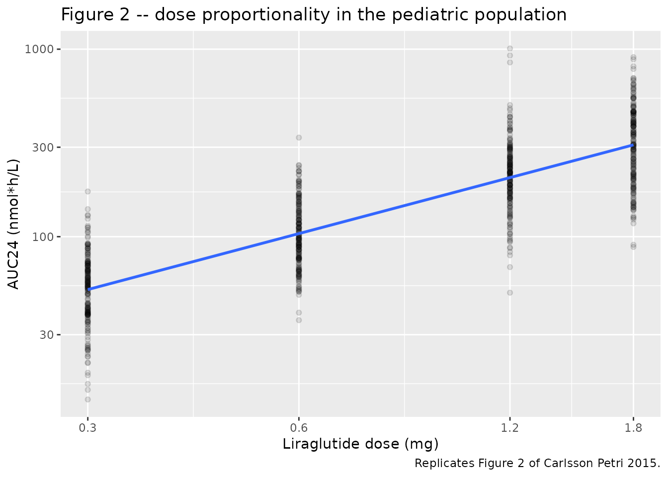
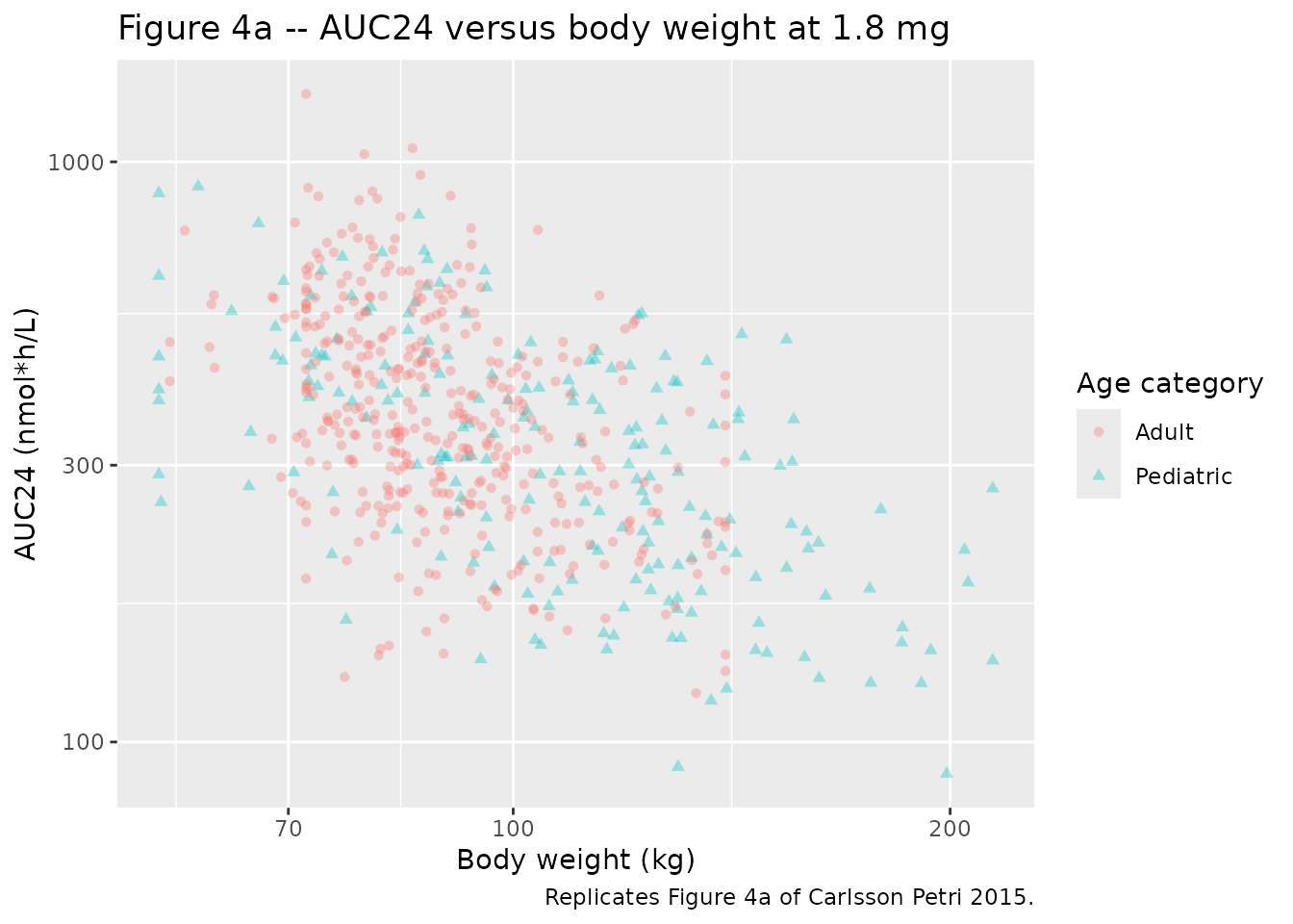
Figure 4a – AUC24 versus body weight by age category

# Replicates Figure 4a of Carlsson Petri 2015: AUC24 versus body weight at
# 1.8 mg once daily, pediatric versus adult. The published figure notes that
# the model-predicted lines for the two age categories are "completely
# superimposed".
nca_tbl |>
  filter(PPTESTCD == "auclast",
         arm %in% c("Trial 1 (pediatric)", "Trial 2 (adult)", "Trial 3 (adult)")) |>
  left_join(distinct(sim, id, WT, CHILD), by = "id") |>
  mutate(`Age category` = ifelse(CHILD == 1, "Pediatric", "Adult")) |>
  ggplot(aes(WT, PPORRES, colour = `Age category`, shape = `Age category`)) +
  geom_point(alpha = 0.35) +
  scale_x_log10() +
  scale_y_log10() +
  labs(
    x = "Body weight (kg)", y = "AUC24 (nmol*h/L)",
    title = "Figure 4a -- AUC24 versus body weight at 1.8 mg",
    caption = "Replicates Figure 4a of Carlsson Petri 2015."
  )

Comparison against the published per-trial exposures

Results reports median (range) CL/F at the 1.8 mg dose for each trial. Methods Sect. 2.2 defines exposure as AUC24 = dose (in nmol) / (CL/F), so the published CL/F medians convert directly to published AUC24 medians – the quantity plotted in Figure 4a.

These published values are empirical Bayes (post-hoc) summaries of 13, 12 and 32 real subjects, not model parameters. They carry that sample’s specific covariate draw and its shrinkage, so they are a deviation check, not a gate.

published_clf <- tibble::tribble(
  ~arm,                  ~clf_median, ~clf_range,
  "Trial 1 (pediatric)", 1.55,        "0.67-3.83",
  "Trial 2 (adult)",     0.91,        "0.59-2.35",
  "Trial 3 (adult)",     1.48,        "1.04-3.72"
)

published_auc <- published_clf |>
  mutate(auclast = mg_to_nmol(1.8) / clf_median) |>
  select(arm, auclast)

cmp <- nlmixr2lib::ncaComparisonTable(
  simulated = nca_tbl |> filter(arm %in% published_auc$arm),
  reference = published_auc,
  by = "arm",
  params = "auclast",
  units = c(auclast = "nmol*h/L"),
  tolerance_pct = 20
)

knitr::kable(
  cmp,
  caption = "Median steady-state AUC0-24 at 1.8 mg: simulated cohort versus the article's post-hoc CL/F medians converted via AUC24 = dose / (CL/F).",
  align = c("l", "l", "r", "r", "r")
)

Median steady-state AUC0-24 at 1.8 mg: simulated cohort versus the article’s post-hoc CL/F medians converted via AUC24 = dose / (CL/F).
NCA parameter	arm	Reference	Simulated	% diff
AUClast (nmol*h/L)	Trial 1 (pediatric)	310	309	-0.0%
AUClast (nmol*h/L)	Trial 2 (adult)	527	408	-22.5%*
AUClast (nmol*h/L)	Trial 3 (adult)	324	319	-1.6%

differs from reference by more than ±20%.

nca_tbl |>
  filter(PPTESTCD == "auclast", arm %in% published_clf$arm) |>
  left_join(distinct(sim, id, arm, cl), by = c("id", "arm")) |>
  group_by(arm) |>
  summarise(
    sim_median = median(cl),
    sim_range = sprintf("%.2f-%.2f", min(cl), max(cl)),
    .groups = "drop"
  ) |>
  left_join(published_clf, by = "arm") |>
  mutate(
    `% diff` = round(100 * (sim_median - clf_median) / clf_median, 1),
    sim_median = round(sim_median, 2)
  ) |>
  select(arm, clf_median, clf_range, sim_median, sim_range, `% diff`) |>
  rename(
    "Trial" = arm,
    "Published median CL/F (L/h)" = clf_median,
    "Published range" = clf_range,
    "Simulated median CL/F (L/h)" = sim_median,
    "Simulated range" = sim_range
  ) |>
  knitr::kable(caption = "Per-trial CL/F at 1.8 mg: the article's post-hoc estimates versus the packaged model's virtual cohorts.")

Per-trial CL/F at 1.8 mg: the article’s post-hoc estimates versus the packaged model’s virtual cohorts.
Trial	Published median CL/F (L/h)	Published range	Simulated median CL/F (L/h)	Simulated range	% diff
Trial 1 (pediatric)	1.55	0.67-3.83	1.55	0.53-5.44	0.0
Trial 2 (adult)	0.91	0.59-2.35	1.17	0.37-3.40	29.1
Trial 3 (adult)	1.48	1.04-3.72	1.50	0.55-3.95	1.7

The simulated Trial 1 and Trial 3 medians track the published post-hoc medians to within 2 %. Trial 2 is the one starred row, and the discrepancy is internal to the article rather than a transcription problem: the article’s own published covariate model, evaluated by hand at Trial 2’s published demographics, disagrees with Trial 2’s published post-hoc median by the same margin.

# The published CL/F equation at Trial 2's published demographics
# (median 83 kg, 50 % female), using only numbers printed in the article.
clf_hat <- function(wt, sexf, child) {
  1.06 * (wt / 90)^0.929 * exp(0.365 * (1 - sexf) + 0.107 * child)
}

tibble::tibble(
  Trial = c("Trial 1 (pediatric)", "Trial 2 (adult)", "Trial 3 (adult)"),
  `Median WT (kg)` = c(106, 83, 96),
  `Female (%)` = c(62, 50, 28),
  `CL/F from the published equation (L/h)` = round(c(
    stats::median(c(rep(clf_hat(106, 1, 1), 62), rep(clf_hat(106, 0, 1), 38))),
    stats::median(c(rep(clf_hat(83, 1, 0), 50), rep(clf_hat(83, 0, 0), 50))),
    stats::median(c(rep(clf_hat(96, 1, 0), 28), rep(clf_hat(96, 0, 0), 72)))
  ), 2),
  `Published post-hoc median CL/F (L/h)` = c(1.55, 0.91, 1.48)
) |>
  mutate(`% diff` = round(100 * (.data[["CL/F from the published equation (L/h)"]] -
                                   .data[["Published post-hoc median CL/F (L/h)"]]) /
                            .data[["Published post-hoc median CL/F (L/h)"]], 1)) |>
  knitr::kable(caption = "The article's own covariate equation evaluated at each trial's published demographics, versus the article's published post-hoc CL/F medians.")

The article’s own covariate equation evaluated at each trial’s published demographics, versus the article’s published post-hoc CL/F medians.
Trial	Median WT (kg)	Female (%)	CL/F from the published equation (L/h)	Published post-hoc median CL/F (L/h)	% diff
Trial 1 (pediatric)	106	62	1.37	1.55	-11.6
Trial 2 (adult)	83	50	1.20	0.91	31.9
Trial 3 (adult)	96	28	1.62	1.48	9.5

Trial 2 is the smallest adult cohort (n = 12) and the only one whose post-hoc median sits more than 20 % away from the article’s own fitted covariate model (+32 %, against +10 % and -12 % for Trials 3 and 1). Note that this hand calculation evaluates the equation at each trial’s median weight, whereas the simulated medians above integrate over the whole weight distribution, so the two columns are not expected to agree exactly; what matters here is that Trial 2 is the outlier under either reading. The packaged model reproduces the equation the authors published rather than that cohort’s shrunken empirical Bayes estimates. No parameter was tuned to close the gap.

Steady-state NCA summary

nca_tbl |>
  # PKNCA already reports tmax relative to the dose at the interval start,
  # so no rebasing is needed.
  filter(PPTESTCD %in% c("cmax", "tmax", "cmin", "auclast", "cav")) |>
  group_by(arm, PPTESTCD) |>
  summarise(median = median(PPORRES), .groups = "drop") |>
  mutate(
    Parameter = nlmixr2lib::ncaParamLabel(
      PPTESTCD,
      units = c(cmax = "nmol/L", cmin = "nmol/L", cav = "nmol/L",
                auclast = "nmol*h/L", tmax = "h")
    ),
    median = signif(median, 3)
  ) |>
  select(Parameter, arm, median) |>
  tidyr::pivot_wider(names_from = arm, values_from = median) |>
  knitr::kable(caption = "Median steady-state NCA parameters by arm (tmax expressed as time since the last dose).")

Median steady-state NCA parameters by arm (tmax expressed as time since the last dose).
Parameter	0.3 mg	0.6 mg	1.2 mg	Trial 1 (pediatric)	Trial 2 (adult)	Trial 3 (adult)
AUClast (nmol*h/L)	55.20	98.60	218.00	309.00	408.00	319.00
Cavg (nmol/L)	2.30	4.11	9.07	12.90	17.00	13.30
Cmax (nmol/L)	2.64	4.78	10.40	14.90	19.10	15.30
Cmin (nmol/L)	1.72	2.99	6.78	9.49	13.40	9.86
Tmax (h)	8.38	8.25	8.25	8.25	8.75	8.25

Assumptions and deviations

Every parameter value comes from the Online Resource (ESM) Table 1, not the main article. The main article prints no parameter estimates at all. The ESM was retrieved from Springer’s static-content endpoint and cross-checked against the EuropePMC supplementaryFiles copy for PMC4449373; the two files are byte-identical.
etalvc is encoded as fixed(0). Methods Sect. 2.2 states that “between-subject variability parameters were included for CL/F and Vd/F (data not shown)”, but ESM Table 1 reports a BSV estimate for CL/F only. The V/F variance is genuinely unpublished, so it is set to a structural zero rather than invented. Simulated between-subject spread in V/F – and therefore in Cmax and tmax – is consequently narrower than the real trials’.
The ESM Table 1 KA unit (“L/h”) is treated as a typographical error and encoded as 1/h. See the scale checks above.
The %CV columns are read on the NONMEM variance scale (omega^2 = (CV/100)^2), settled against the article’s printed 50 % BSV reduction. See the scale checks above.
The BSV row is labelled “CL/F (dose 1.8 mg)” in ESM Table 1. The article describes a plain between-subject variance on CL/F, and no per-dose-level variance components are reported, so the single published value is applied at all dose levels. If the authors did estimate dose-level-specific variances, only the 1.8 mg one is recoverable from the published record.
Body-weight distributions are assumed truncated log-normal with each trial’s published median as the geometric mean and a sdlog chosen so the draws span the published range; draws are then clipped to that range. The article publishes only median and range (Table 1), not the distribution.
Sex is assigned deterministically to match each trial’s published female percentage exactly rather than being drawn at random.
Age is not a model covariate beyond the pediatric/adult indicator. Methods Sect. 2.2 explains that the narrow pediatric age range and the 17-to-33-year gap to the youngest adult made a continuous age covariate infeasible.
Race and ethnicity are not in the model. The article does not report a race/ethnicity distribution for these three trials and notes that prior adult analyses found no effect.
Dose escalation is not simulated. All arms are simulated as 12 once-daily doses at a fixed level, which is what the steady-state comparisons require. The real Trial 1 escalated weekly and some subjects never reached 1.8 mg; Figure 4a of the article normalises those subjects’ AUC24 to a 1.8 mg dose, which is equivalent to the fixed-dose simulation used here because the model is exactly dose-proportional.
The published protocol deviations (0.9 mg and 1.5 mg observations) are not reproduced; they contributed observations to the fit but are not part of any published summary this vignette compares against.
No non-paper-derived parameter values are used. Every ini() entry traces to ESM Table 1.