Losartan whole-body PBPK/PD (Tensil 2026)
Source:vignettes/articles/Tensil_2026_losartan_pbpk.Rmd
Tensil_2026_losartan_pbpk.RmdThe model
Tensil_2026_losartan_pbpk is a whole-body
physiologically based pharmacokinetic/pharmacodynamic model of losartan,
its active CYP2C9 metabolite E3174 (losartan carboxylic acid) and the
E3174 glucuronide L158, built by Tensil, Myshkina and Koenig (2026) from
25 curated clinical studies and distributed by the authors as SBML under
CC-BY.
mod <- rxode2::rxode(readModelDb("Tensil_2026_losartan_pbpk"))
length(mod$state)
#> [1] 49
The 49 ODEs are organised as a systemic circulation (venous, arterial, portal and hepatic-venous plasma pools, plus lung and a lumped rest-of-body) linking three pharmacokinetic submodels and one pharmacodynamic submodel:
-
Intestine. Oral losartan dissolves into the gut
lumen at
ka_dis_los. Of the flux leaving the lumen, 60% (f_los_abs) enters the enterocytes and 40% is excreted in feces. P-glycoprotein (ABCB1) effluxes losartan from the enterocytes back to the lumen; the remainder passes to gut plasma. E3174 and L158 that reach the lumen in bile are excreted in feces. -
Liver. Losartan is taken up into liver tissue,
converted to E3174 by CYP2C9 (Michaelis-Menten; the covariate
CYP2C9scales the Vmax), and E3174 to L158 (first order). E3174 and L158 are exported back to plasma, and all three species are secreted into bile, which empties into the gut lumen. -
Kidney. First-order urinary excretion of all three
species from kidney plasma, scaled by
RENALFUNC_REL. - RAAS. One Emax term on venous E3174 raises renin secretion (up to six-fold) and suppresses aldosterone secretion. Renin converts a constant angiotensinogen pool to angiotensin I, which turns over to angiotensin II, and systolic, diastolic and mean arterial pressure move in proportion to the aldosterone deviation from baseline.
Hepatic impairment (HEPFUNC_REL) shrinks the
metabolising liver volume and shunts portal and hepatic-arterial blood
past the liver; body weight (WT) scales every organ volume
and blood flow.
A note on units and dosing. Drug states are
concentrations in umol/L (cumulative urine and feces pools are
amounts in umol) and the RAAS hormones are in pmol/L; the outputs
Cc, Cc_e3174 and Cc_l158 are
venous plasma concentrations in nmol/L, matching the
paper’s figures. Doses (mg) must go into depot (oral),
depot_iv (intravenous losartan) or
depot_iv_e3174 (intravenous E3174) and never directly into
a plasma or tissue compartment. Model time is in
minutes.
Population
pop <- mod$population
data.frame(Field = names(pop), Value = vapply(pop, as.character, character(1))) |>
knitr::kable(row.names = FALSE)| Field | Value |
|---|---|
| species | human |
| n_subjects | NA |
| n_studies | 25 |
| age_range | adults; not tabulated per study in the source |
| weight_range | study-specific mean bodyweight where reported (52-84.6 kg across Supplementary Table S5); 75 kg reference individual otherwise |
| sex_female_pct | NA |
| disease_state | Healthy volunteers, CYP2C9 and ABCB1 genotyped volunteers, and subjects with hepatic (cirrhosis) or renal impairment (Table 1). Animal, pediatric, single-patient, cocktail and combination studies were excluded (Methods Section 2.1). |
| dose_range | Oral losartan 2-200 mg single and multiple dose (Table 1); intravenous losartan 10-30 mg and intravenous E3174 10-20 mg (FDA 1995 studies 60 and 67, Lo 1995). |
| regions | not reported |
| notes | Deterministic typical-individual model. Methods Section 2.3 states that ‘all simulations were performed deterministically using the optimized parameter set representing the typical (mean) individual’ and that inter-individual variability was NOT included, so no IIV and no residual-error model are reported and none are invented here. Data were curated into PK-DB (identifiers in Table 1) from a PubMed and PKPDAI search screening 787 records down to 25 studies. Parameters were fitted sequentially by weighted least squares with 100 multi-start local optimisation runs - pharmacokinetic first (12 parameters, Table S2), then pharmacodynamic (4 parameters, Table S3). Pharmacodynamic data (renin, angiotensin, aldosterone, blood pressure) came from a smaller subset of studies and showed high between-study variability (Discussion). |
The model is deterministic. Methods Section 2.3
states that all simulations were “performed deterministically using the
optimized parameter set representing the typical (mean) individual” and
that inter-individual variability was not included, so the model carries
no IIV and no residual-error estimate, and propSd is fixed
at zero. Every simulation below is a single typical individual per
scenario.
Source trace
| Quantity | Parameters | Source |
|---|---|---|
| Fractional organ volumes (gut, kidney, liver, lung) |
fvgu, fvki, fvli,
fvlu
|
Methods 2.3 (1.71%, 0.44%, 2.10%, 0.76%); Table S7 |
| Fractional blood-pool volumes |
fvar, fvve
|
Table S7 (0.0257, 0.0514 L/kg) |
| Portal and hepatic-venous fractional volumes |
fvpo, fvhv
|
Archived SBML FVpo, FVhv (not
tabulated) |
| Fractional blood flows |
fqgu, fqh, fqki,
fqlu
|
Methods 2.3 (18.00%, 21.50%, 19.00%, 100%); Table S7 |
| Cardiac output, hematocrit |
covbw, hct
|
Table S7 COBW (1.55 mL/s/kg; SBML 1.548),
HCT (0.51) |
| Blood fraction, cardiac function, enterocyte and RAAS volumes |
fblood, fcardio, v_entero,
vplasma
|
Archived SBML Fblood, f_cardiac_function,
GU__Ventero, Vplasma
|
| Molecular weights |
mr_los, mr_e3174
|
Archived SBML Mr_los, Mr_e3174
|
| Partition coefficient, tissue distribution |
kp_los, ftissue_los
|
Table S2 (3.262; 0.145 L/min); Methods 2.3 |
| Dissolution, absorption, absorbed fraction |
ka_dis_los, losabs_k,
f_los_abs
|
Table S7 (2 /h); Table S2 (0.036 /min); Table S7 (0.6) |
| P-gp efflux, fecal metabolite excretion |
f_losefl_k, metexc_k
|
Table S2 (1.020; 2.696e-5 /min) |
| Uptake and P-gp activity scalars |
f_oatp2b1, f_abcb1
|
Table S7 (1, 1) |
| Hepatic CYP2C9 metabolism |
los2e3174_vmax, los2e3174_km
|
Table S2 (7.251e-4 mmol/min/L); Table S7 Km 0.0011 mmol/L (literature) |
| E3174 to L158, E3174 export, biliary export |
e3174l158_k, li_e3174ex_k,
mbiex_k
|
Table S2 (1.134e-3; 0.011; 0.066 /min) |
| Hepatic losartan uptake, L158 export |
losim_k, li_l158ex_k
|
Archived SBML LI__LOSIM_k, LI__L158EX_k (1
/min; not fitted) |
| Renal excretion |
ki_losex_k, ki_e3174ex_k,
ki_l158ex_k
|
Table S2 (0.077; 0.029; 0.289 /min) |
| RAAS fitted parameters |
anggen2ang1_k, e50_e3174,
aldsec_k, bp_ald_fe
|
Table S3 (0.100 L/min; 2.911e-4 mmol/L; -; 0.312);
aldsec_k from Table S7 (1.01e-6 mmol/min) – see Errata |
| RAAS fixed parameters |
rensec_k, rensec_fa_e3174
|
Table S7 (0.1 mmol/min; 5) |
| Baseline hormones |
ren_ref, ang1_ref, ang2_ref,
ald_ref, anggen_ref
|
Archived SBML *_ref (1, 10, 8, 250, 10 pmol/L) |
| Baseline blood pressure |
sbp_ref, dbp_ref
|
Results 3.2 (120/80 mmHg) |
| Scenario covariates |
WT, RENALFUNC_REL,
HEPFUNC_REL, CYP2C9
|
Table S7 (BW, KI__f_renal_function,
LI__f_cyp2c9); f_cirrhosis from the archived
SBML and Tables S5/S6; per-study values Table S5 |
None of the rate laws or ODEs are printed in the manuscript or the
Supplementary Materials. They were taken from the authors’ archived SBML
model, which Methods Section 2.3 cites as shared on Zenodo at v0.8.0
(reference 53: 10.5281/zenodo.18213663;
file models/losartan_body_flat.md of the 0.8.0 release of
github.com/matthiaskoenig/losartan-model). Every parameter value of that
release agrees with Supplementary Tables S2, S3 and S7 to the printed
precision, apart from the ALDSEC_k entry of Table S3 (see
Errata); the full-precision SBML values are used in
ini().
Simulation helper
# Time is in minutes. Observations are placed on the `venous` ODE state; rxode2
# returns every algebraic observable (Cc, Cc_e3174, SBP, ...) as a column on
# those rows.
sim_los <- function(dose_mg = 50, route = "depot", hours = 48, by_min = 5,
                    wt = 75, renal = 1, hep = 1, cyp2c9 = 1, model = mod,
                    times = NULL, tight = FALSE) {
  tt <- if (is.null(times)) seq(0, hours * 60, by = by_min) else times
  ev <- rbind(
    data.frame(time = 0, amt = dose_mg, evid = 1L, cmt = route),
    data.frame(time = tt, amt = NA_real_, evid = 0L, cmt = "venous")
  )
  ev$WT <- wt
  ev$RENALFUNC_REL <- renal
  ev$HEPFUNC_REL <- hep
  ev$CYP2C9 <- cyp2c9
  out <- if (tight) {
    rxode2::rxSolve(model, ev, returnType = "data.frame", atol = 1e-12, rtol = 1e-10)
  } else {
    rxode2::rxSolve(model, ev, returnType = "data.frame")
  }
  out <- as.data.frame(out)
  out$hour <- out$time / 60
  out
}

# Trapezoidal AUC on the dense simulation grid (summary use only; the PKNCA
# section below is the NCA of record).
trap <- function(t, y) sum(diff(t) * (head(y, -1) + tail(y, -1)) / 2)
Exact reproduction of the authors’ model
The strongest check available for a model distributed as SBML is to
simulate that SBML directly and compare. The table below holds reference
values computed with libroadrunner 2.11 from the authors’ archived
losartan_body_flat.xml (release 0.8.0) at tolerances 1e-14
absolute / 1e-10 relative, for ten scenarios covering every route and
every covariate: oral 10, 50 and 100 mg; 50 mg with cirrhosis
(f_cirrhosis 0.67, the FDA 1995 study 67 value), renal
impairment (KI__f_renal_function 0.14), CYP2C9 activity
0.17, ABCB1 activity 0.306 and body weight 60 kg; intravenous losartan
30 mg and intravenous E3174 20 mg. Concentrations are in nmol/L, renin
and aldosterone in pmol/L, SBP in mmHg and cumulative urinary E3174 in
umol.
rr <- tibble::tribble(
  ~scenario, ~time, ~Cc, ~Cc_e3174, ~Cc_l158, ~renin, ~aldosterone, ~SBP, ~urine_e3174,
  "po50", 60, 400.9947, 167.9322, 8.349906, 2.829307, 161.0193, 106.6743, 0.02697759,
  "po50", 180, 101.7525, 501.1334,  9.45803, 4.162898, 91.82095, 96.31116, 0.4765545,
  "po50", 720, 21.57749, 108.7675, 0.8303907, 2.360137, 181.8482, 109.7936, 1.789382,
  "po10", 60, 74.78837, 35.72772, 1.779888, 1.546629, 223.6971, 116.0609, 0.005694748,
  "po10", 180, 19.52231, 104.1864, 1.931643,  2.31795, 184.0634, 110.1254, 0.100279,
  "po10", 720, 4.075586, 21.46125, 0.1586794, 1.343343, 232.7842, 117.4218, 0.3676898,
  "po100", 60, 876.0789, 307.5659, 15.24276, 3.568878, 124.2178, 101.1629, 0.05008329,
  "po100", 180, 215.4605, 945.5142, 18.32171,  4.82308, 58.83488, 91.37118, 0.8834033,
  "po100", 720, 46.58667, 221.6223, 1.765669, 3.161346, 141.7627, 103.7904, 3.439145,
  "po50_cirr067", 60,  727.248, 73.25295, 4.417902, 2.005322, 201.5384, 112.7424, 0.01138136,
  "po50_cirr067", 180, 234.4563, 280.9034, 7.406594, 3.455552, 127.3435,  101.631, 0.2383445,
  "po50_cirr067", 720, 81.10768, 169.6968, 1.339973,  2.84145, 157.8574, 106.2008, 1.393155,
  "po50_renal014", 60,  411.142, 173.6355, 9.922634, 2.868221, 159.1443, 106.3935, 0.0038965,
  "po50_renal014", 180, 105.6414, 576.6098, 17.51916,   4.3227, 83.90742, 95.12603, 0.07318147,
  "po50_renal014", 720, 23.02296, 213.0373, 1.808677, 3.113004, 144.2097, 104.1569, 0.3432374,
  "po50_cyp017", 60, 671.0298, 49.42683, 2.460787, 1.725799, 215.0347, 114.7636, 0.007882573,
  "po50_cyp017", 180, 236.1442, 178.2883, 3.814194, 2.899266, 155.1204, 105.7909, 0.1542534,
  "po50_cyp017", 720, 73.15641, 73.88037, 0.7720712,  2.01219, 199.3283, 112.4114, 0.7614893,
  "po50_abcb1_0306", 60, 544.9191, 204.0262, 10.19727, 3.060459, 149.6927,  104.978, 0.03199825,
  "po50_abcb1_0306", 180, 122.6635, 635.2368, 11.93637, 4.428858, 78.51121,  94.3179, 0.6009125,
  "po50_abcb1_0306", 720, 27.97719, 137.2101, 1.071993, 2.601863, 169.7521, 107.9821, 2.237123,
  "po50_bw60", 60, 448.4444, 184.0536, 9.176471, 2.936891, 155.7647, 105.8874, 0.02335062,
  "po50_bw60", 180, 134.2359, 590.1041, 11.57109, 4.348386, 82.57712, 94.92681, 0.4357186,
  "po50_bw60", 720, 31.08124, 146.4356, 1.183895, 2.673518, 166.1722,  107.446, 1.746884,
  "iv30", 60, 131.9622,  482.696, 18.00487, 4.119123, 94.23357, 96.67248, 0.1608347,
  "iv30", 180, 84.67303, 400.3066, 4.034879, 3.894985, 105.0876, 98.29797, 0.6649228,
  "iv30", 720, 46.95715, 160.8498, 1.680699, 2.779617,  160.927, 106.6605, 1.928968,
  "iv20_e3174", 60,        0, 6713.611, 6.658412,  5.79223, 10.33153, 84.10734, 4.297814,
  "iv20_e3174", 180,        0, 3845.284, 5.915158, 5.648153, 17.49886, 85.18071, 10.04074,
  "iv20_e3174", 720,        0, 313.2995, 0.4934254, 3.591941, 120.0445, 100.5379, 17.11368
)

scenarios <- list(
  po10 = list(dose_mg = 10),
  po50 = list(dose_mg = 50),
  po100 = list(dose_mg = 100),
  po50_cirr067 = list(hep = 1 - 0.67),
  po50_renal014 = list(renal = 0.14),
  po50_cyp017 = list(cyp2c9 = 0.17),
  po50_abcb1_0306 = list(model = mod |> rxode2::ini(f_abcb1 = 0.306)),
  po50_bw60 = list(wt = 60),
  iv30 = list(dose_mg = 30, route = "depot_iv"),
  iv20_e3174 = list(dose_mg = 20, route = "depot_iv_e3174")
)
#> ℹ change initial estimate of `f_abcb1` to `0.306`

ours <- bind_rows(lapply(names(scenarios), function(nm) {
  args <- c(scenarios[[nm]], list(times = c(60, 180, 720), tight = TRUE))
  do.call(sim_los, args) |>
    mutate(scenario = nm) |>
    select(scenario, time, Cc, Cc_e3174, Cc_l158, renin, aldosterone, SBP, urine_e3174)
}))

cmp <- rr |>
  pivot_longer(-c(scenario, time), names_to = "output", values_to = "roadrunner") |>
  inner_join(
    ours |> pivot_longer(-c(scenario, time), names_to = "output", values_to = "rxode2"),
    by = c("scenario", "time", "output")
  ) |>
  filter(roadrunner != 0) |>
  mutate(rel_diff = abs(rxode2 / roadrunner - 1))

cmp |>
  group_by(output) |>
  summarise(n = n(), max_rel_diff = max(rel_diff)) |>
  rename("Output" = output, "Values compared" = n, "Max relative difference" = max_rel_diff) |>
knitr::kable(digits = 10)| Output | Values compared | Max relative difference |
|---|---|---|
| Cc | 27 | 3.918e-07 |
| Cc_e3174 | 30 | 3.367e-07 |
| Cc_l158 | 30 | 4.099e-07 |
| SBP | 30 | 4.492e-07 |
| aldosterone | 30 | 3.010e-07 |
| renin | 30 | 2.196e-07 |
| urine_e3174 | 30 | 2.442e-07 |
stopifnot(
  nrow(cmp) == 7 * 30 - 3, # the three losartan values of the IV-E3174 arm are exactly 0
  max(cmp$rel_diff) < 1e-4 # measured ~4e-7 at these tolerances
)
All 207 non-zero values agree to better than 1e-4, so every flow, volume, rate law and scenario scalar of the SBML has been carried over faithfully.
Mass balance
Losartan, E3174 and L158 are interconverted one-to-one, so the total drug-related amount in the body plus what has been excreted must equal the dose at every time.
mb <- sim_los(50, hours = 24 * 7, by_min = 60, tight = TRUE)
dose_umol <- 50 / 422.911 * 1000
species_amount <- function(s, sfx) {
  with(s, get(paste0("gut_lumen", sfx)) * vgu +
    get(paste0("gut_plasma", sfx)) * vgu_plasma +
    get(paste0("portal", sfx)) * vpo +
    get(paste0("liver_plasma", sfx)) * vli_plasma +
    get(paste0("liver", sfx)) * vli_tissue +
    get(paste0("hepatic_vein", sfx)) * vhv +
    get(paste0("kidney_plasma", sfx)) * vki_plasma +
    get(paste0("lung_plasma", sfx)) * vlu_plasma +
    get(paste0("rest_plasma", sfx)) * vre_plasma +
    get(paste0("venous", sfx)) * vve +
    get(paste0("arterial", sfx)) * var_ +
    get(paste0("urine", sfx)) + get(paste0("feces", sfx)))
}
mb <- mb |>
  mutate(
    total = 1000 * depot / 422.911 + gut * 1 +
      lung * vlu_tissue + rest * vre_tissue +
      species_amount(mb, "") + species_amount(mb, "_e3174") + species_amount(mb, "_l158")
  )
stopifnot(max(abs(mb$total / dose_umol - 1)) < 1e-6)

last <- tail(mb, 1)
recovery <- tibble::tibble(
  Route = c("Urine", "Urine", "Urine", "Feces", "Feces", "Feces"),
  Species = rep(c("losartan", "E3174", "L158"), 2),
  `Percent of dose at 7 days` = 100 * c(
    last$urine, last$urine_e3174, last$urine_l158,
    last$feces, last$feces_e3174, last$feces_l158
  ) / dose_umol
)
knitr::kable(recovery, digits = 2)| Route | Species | Percent of dose at 7 days |
|---|---|---|
| Urine | losartan | 1.70 |
| Urine | E3174 | 2.10 |
| Urine | L158 | 0.26 |
| Feces | losartan | 59.90 |
| Feces | E3174 | 8.14 |
| Feces | L158 | 0.08 |
The model conserves mass to integrator precision. It routes about 60% of the dose to feces as unchanged losartan – the 40% of the luminal flux that is never absorbed, plus losartan returned in bile – and another 8% as E3174, but only a few percent to urine. Figure 2 of the paper quotes clinical recovery of 49-58% of the dose in feces and 5-12% (losartan) and 6-7% (E3174) in urine, so the model somewhat over-predicts fecal and under-predicts urinary recovery; see the Errata.
Dose dependency (Figure 3)
doses <- c(10, 25, 50, 75, 100)
dd <- bind_rows(lapply(doses, function(d) sim_los(d, hours = 36) |> mutate(dose_mg = d)))

dd |>
  select(hour, dose_mg, Cc, Cc_e3174, Cc_l158, renin, ang1, aldosterone, SBP, DBP) |>
  pivot_longer(-c(hour, dose_mg)) |>
  mutate(name = factor(name, levels = c("Cc", "Cc_e3174", "Cc_l158", "renin", "ang1",
                                        "aldosterone", "SBP", "DBP"))) |>
  ggplot(aes(hour, value, colour = factor(dose_mg))) +
  geom_line() +
  facet_wrap(~name, scales = "free_y", ncol = 4) +
  labs(x = "Time (h)", y = "Concentration (nmol/L or pmol/L) / pressure (mmHg)",
       colour = "Dose (mg)",
       title = "Replicates Figure 3B of Tensil 2026")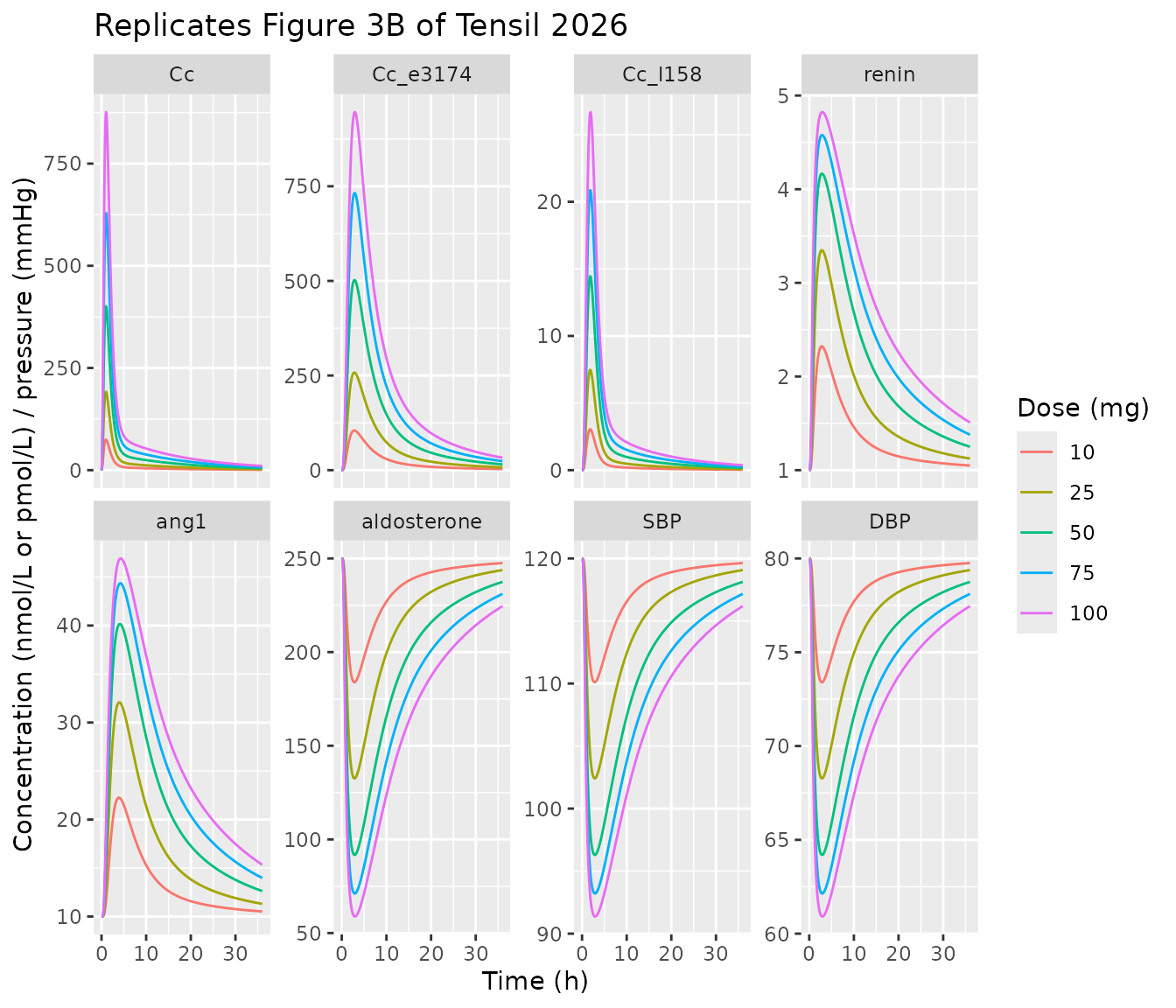
dose_tab <- dd |>
  group_by(dose_mg) |>
  summarise(
    auc_los = trap(hour, Cc) / 1000,
    auc_e3174 = trap(hour, Cc_e3174) / 1000,
    cmax_los = max(Cc) / 1000,
    cmax_e3174 = max(Cc_e3174) / 1000,
    ratio = auc_e3174 / auc_los,
    min_sbp = min(SBP),
    min_dbp = min(DBP),
    max_renin = max(renin),
    min_ald = min(aldosterone)
  )
dose_tab |>
  rename(
    "Dose (mg)" = dose_mg, "Losartan AUC0-36 (umol*h/L)" = auc_los,
    "E3174 AUC0-36 (umol*h/L)" = auc_e3174, "Losartan Cmax (umol/L)" = cmax_los,
    "E3174 Cmax (umol/L)" = cmax_e3174, "E3174/losartan AUC ratio" = ratio,
    "Min SBP (mmHg)" = min_sbp, "Min DBP (mmHg)" = min_dbp,
    "Max renin (pmol/L)" = max_renin, "Min aldosterone (pmol/L)" = min_ald
  ) |>
knitr::kable(digits = 3)| Dose (mg) | Losartan AUC0-36 (umol*h/L) | E3174 AUC0-36 (umol*h/L) | Losartan Cmax (umol/L) | E3174 Cmax (umol/L) | E3174/losartan AUC ratio | Min SBP (mmHg) | Min DBP (mmHg) | Max renin (pmol/L) | Min aldosterone (pmol/L) |
|---|---|---|---|---|---|---|---|---|---|
| 10 | 0.244 | 0.852 | 0.075 | 0.105 | 3.488 | 110.100 | 73.400 | 2.322 | 183.895 |
| 25 | 0.623 | 2.120 | 0.192 | 0.258 | 3.402 | 102.414 | 68.276 | 3.349 | 132.569 |
| 50 | 1.292 | 4.208 | 0.401 | 0.502 | 3.258 | 96.297 | 64.198 | 4.166 | 91.726 |
| 75 | 2.011 | 6.261 | 0.629 | 0.732 | 3.114 | 93.211 | 62.141 | 4.578 | 71.120 |
| 100 | 2.785 | 8.274 | 0.876 | 0.946 | 2.971 | 91.370 | 60.913 | 4.824 | 58.826 |
stopifnot(
  # "a decreasing E3174/losartan ratio at higher doses" (Section 3.3) --
  # saturable CYP2C9 metabolism.
  all(diff(dose_tab$ratio) < 0),
  # "nonlinear increases in AUC and Cmax": losartan AUC rises more than
  # dose-proportionally.
  dose_tab$auc_los[dose_tab$dose_mg == 100] / dose_tab$auc_los[dose_tab$dose_mg == 10] > 10,
  # Stronger suppression of aldosterone and blood pressure, and larger renin
  # rise, at higher doses.
  all(diff(dose_tab$min_sbp) < 0), all(diff(dose_tab$min_ald) < 0),
  all(diff(dose_tab$max_renin) > 0)
)
Figure 3D plots the minimum SBP and DBP against dose. The model gives the values read off that panel at 50 mg (about 96 and 64 mmHg) and the 10-100 mg span (about 110 to 91 mmHg systolic):
fig3d <- tibble::tribble(
  ~dose_mg, ~pressure, ~figure,
  10, "SBP", 110,
  50, "SBP", 96,
  100, "SBP", 91.5,
  10, "DBP", 73.5,
  50, "DBP", 64,
  100, "DBP", 61
)
fig3d_cmp <- fig3d |>
  left_join(
    dose_tab |>
      select(dose_mg, SBP = min_sbp, DBP = min_dbp) |>
      pivot_longer(-dose_mg, names_to = "pressure", values_to = "model"),
    by = c("dose_mg", "pressure")
  ) |>
  mutate(diff_mmHg = model - figure)
fig3d_cmp |>
  rename("Dose (mg)" = dose_mg, "Pressure" = pressure,
         "Figure 3D read-off (mmHg)" = figure, "Model (mmHg)" = model,
         "Difference (mmHg)" = diff_mmHg) |>
knitr::kable(digits = 1)| Dose (mg) | Pressure | Figure 3D read-off (mmHg) | Model (mmHg) | Difference (mmHg) |
|---|---|---|---|---|
| 10 | SBP | 110.0 | 110.1 | 0.1 |
| 50 | SBP | 96.0 | 96.3 | 0.3 |
| 100 | SBP | 91.5 | 91.4 | -0.1 |
| 10 | DBP | 73.5 | 73.4 | -0.1 |
| 50 | DBP | 64.0 | 64.2 | 0.2 |
| 100 | DBP | 61.0 | 60.9 | -0.1 |
Hepatic impairment (Figure 4)
cirr <- c(0, 0.3, 0.5, 0.67, 0.8, 0.9)
hep <- bind_rows(lapply(cirr, function(f) sim_los(50, hours = 48, hep = 1 - f) |>
  mutate(f_cirrhosis = f)))

hep |>
  select(hour, f_cirrhosis, Cc, Cc_e3174, SBP) |>
  pivot_longer(-c(hour, f_cirrhosis)) |>
  ggplot(aes(hour, value, colour = factor(f_cirrhosis))) +
  geom_line() +
  facet_wrap(~name, scales = "free_y") +
  labs(x = "Time (h)", y = NULL, colour = "f_cirrhosis",
       title = "Replicates Figure 4B of Tensil 2026 (50 mg)")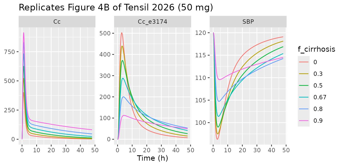
hep_tab <- hep |>
  group_by(f_cirrhosis) |>
  summarise(auc_los = trap(hour, Cc) / 1000, auc_e3174 = trap(hour, Cc_e3174) / 1000,
            ratio = auc_e3174 / auc_los, min_sbp = min(SBP),
            feces_los = 100 * last(feces) / dose_umol)
hep_tab |>
  rename("f_cirrhosis" = f_cirrhosis, "Losartan AUC (umol*h/L)" = auc_los,
         "E3174 AUC (umol*h/L)" = auc_e3174, "E3174/losartan" = ratio,
         "Min SBP (mmHg)" = min_sbp, "Fecal losartan (% dose)" = feces_los) |>
knitr::kable(digits = 3)| f_cirrhosis | Losartan AUC (umol*h/L) | E3174 AUC (umol*h/L) | E3174/losartan | Min SBP (mmHg) | Fecal losartan (% dose) |
|---|---|---|---|---|---|
| 0.00 | 1.332 | 4.337 | 3.257 | 96.297 | 59.856 |
| 0.30 | 2.036 | 5.034 | 2.473 | 97.479 | 59.753 |
| 0.50 | 2.847 | 5.473 | 1.922 | 99.008 | 59.598 |
| 0.67 | 4.003 | 5.571 | 1.392 | 101.384 | 59.333 |
| 0.80 | 5.473 | 5.016 | 0.916 | 104.745 | 58.939 |
| 0.90 | 7.277 | 3.571 | 0.491 | 109.552 | 58.392 |
stopifnot(
  # "As cirrhosis severity increases, losartan plasma ... concentrations rise,
  # while ... the E3174/losartan ratio decrease[s]" (Section 3.4).
  all(diff(hep_tab$auc_los) > 0), all(diff(hep_tab$ratio) < 0),
  # "Fecal excretion remains largely unchanged".
  diff(range(hep_tab$feces_los)) < 5,
  # Attenuated blood-pressure response in severe cirrhosis.
  hep_tab$min_sbp[hep_tab$f_cirrhosis == 0.9] > hep_tab$min_sbp[hep_tab$f_cirrhosis == 0]
)
Renal impairment (Figure 5)
renal_lv <- c(1, 0.95, 0.5, 0.14)
ren <- bind_rows(lapply(renal_lv, function(r) sim_los(50, hours = 48, renal = r) |>
  mutate(renal = r)))
ren_tab <- ren |>
  group_by(renal) |>
  summarise(auc_los = trap(hour, Cc) / 1000, auc_e3174 = trap(hour, Cc_e3174) / 1000,
            urine_los = last(urine), urine_e3174 = last(urine_e3174),
            min_sbp = min(SBP)) |>
  arrange(desc(renal))
ren_tab |>
  rename("Relative renal function" = renal, "Losartan AUC (umol*h/L)" = auc_los,
         "E3174 AUC (umol*h/L)" = auc_e3174, "Urinary losartan (umol)" = urine_los,
         "Urinary E3174 (umol)" = urine_e3174, "Min SBP (mmHg)" = min_sbp) |>
knitr::kable(digits = 3)| Relative renal function | Losartan AUC (umol*h/L) | E3174 AUC (umol*h/L) | Urinary losartan (umol) | Urinary E3174 (umol) | Min SBP (mmHg) |
|---|---|---|---|---|---|
| 1.00 | 1.332 | 4.337 | 1.963 | 2.417 | 96.297 |
| 0.95 | 1.335 | 4.429 | 1.871 | 2.346 | 96.231 |
| 0.50 | 1.367 | 5.463 | 1.017 | 1.528 | 95.622 |
| 0.14 | 1.395 | 6.682 | 0.292 | 0.525 | 95.097 |
stopifnot(
  # "losartan plasma concentrations remain largely unchanged, whereas E3174
  # levels increase, accompanied by reduced urinary excretion of both"
  # (Section 3.5).
  diff(range(ren_tab$auc_los)) / ren_tab$auc_los[1] < 0.1,
  all(diff(ren_tab$auc_e3174) > 0),
  all(diff(ren_tab$urine_los) < 0), all(diff(ren_tab$urine_e3174) < 0),
  # "impaired renal function amplifies losartan's antihypertensive effects".
  all(diff(ren_tab$min_sbp) < 0)
)
ABCB1 activity (Figure 6)
ABCB1 activity is a scaling parameter (f_abcb1, 1 =
reference) rather than a covariate. The Shin 2020 simulation uses 1.0,
0.653 and 0.306 for its three diplotype groups (Supplementary Table S5;
Section 3.6 names the GG/CC, GT/CT and TT/TT diplotypes).
abcb1_lv <- c(1, 0.653, 0.306)
abc <- bind_rows(lapply(abcb1_lv, function(a) {
  sim_los(50, hours = 48, model = mod |> rxode2::ini(f_abcb1 = a)) |> mutate(abcb1 = a)
}))
#> ℹ change initial estimate of `f_abcb1` to `1`
#> ℹ change initial estimate of `f_abcb1` to `0.653`
#> ℹ change initial estimate of `f_abcb1` to `0.306`
abc_tab <- abc |>
  group_by(abcb1) |>
  summarise(auc_los = trap(hour, Cc) / 1000, auc_e3174 = trap(hour, Cc_e3174) / 1000,
            feces_los = 100 * last(feces) / dose_umol, min_sbp = min(SBP)) |>
  arrange(desc(abcb1))
abc_tab |>
  rename("ABCB1 activity" = abcb1, "Losartan AUC (umol*h/L)" = auc_los,
         "E3174 AUC (umol*h/L)" = auc_e3174, "Fecal losartan (% dose)" = feces_los,
         "Min SBP (mmHg)" = min_sbp) |>
knitr::kable(digits = 3)| ABCB1 activity | Losartan AUC (umol*h/L) | E3174 AUC (umol*h/L) | Fecal losartan (% dose) | Min SBP (mmHg) |
|---|---|---|---|---|
| 1.000 | 1.332 | 4.337 | 59.856 | 96.297 |
| 0.653 | 1.503 | 4.836 | 55.196 | 95.333 |
| 0.306 | 1.727 | 5.466 | 49.304 | 94.289 |
stopifnot(
  # "reduced ABCB1 activity leads to increased plasma ... concentrations of
  # both compounds, while fecal excretion of losartan declines" (Section 3.6).
  all(diff(abc_tab$auc_los) > 0), all(diff(abc_tab$auc_e3174) > 0),
  all(diff(abc_tab$feces_los) < 0),
  # Only a slight enhancement of the blood-pressure effect.
  abs(abc_tab$min_sbp[3] - abc_tab$min_sbp[1]) < 5
)
CYP2C9 activity (Figure 7)
The per-study simulations assign a CYP2C9 activity to each genotype group (Supplementary Table S5); for example Li 2009 uses 1.0, 0.525 and 0.17 for its three groups. The paper does not print which diplotype each value belongs to.
cyp_lv <- c(1, 0.8, 0.585, 0.525, 0.385, 0.17)
cyp <- bind_rows(lapply(cyp_lv, function(a) sim_los(50, hours = 48, cyp2c9 = a) |>
  mutate(cyp2c9 = a)))

cyp |>
  select(hour, cyp2c9, Cc, Cc_e3174, SBP) |>
  pivot_longer(-c(hour, cyp2c9)) |>
  ggplot(aes(hour, value, colour = factor(cyp2c9))) +
  geom_line() +
  facet_wrap(~name, scales = "free_y") +
  labs(x = "Time (h)", y = NULL, colour = "CYP2C9 activity",
       title = "Replicates Figure 7B of Tensil 2026 (50 mg)")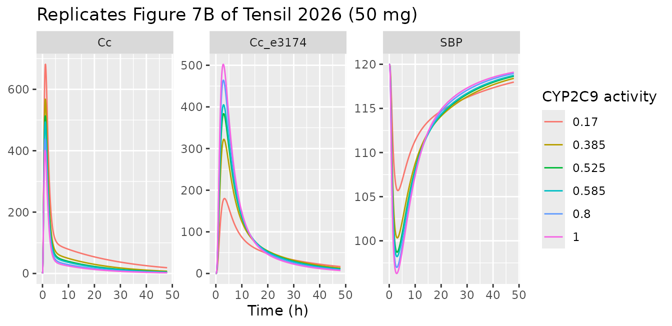
cyp_tab <- cyp |>
  group_by(cyp2c9) |>
  summarise(auc_los = trap(hour, Cc) / 1000, auc_e3174 = trap(hour, Cc_e3174) / 1000,
            min_sbp = min(SBP)) |>
  arrange(desc(cyp2c9)) |>
  mutate(auc_los_ratio = auc_los / auc_los[1])
cyp_tab |>
  rename("CYP2C9 activity" = cyp2c9, "Losartan AUC (umol*h/L)" = auc_los,
         "E3174 AUC (umol*h/L)" = auc_e3174, "Min SBP (mmHg)" = min_sbp,
         "Losartan AUC ratio vs activity 1" = auc_los_ratio) |>
knitr::kable(digits = 3)| CYP2C9 activity | Losartan AUC (umol*h/L) | E3174 AUC (umol*h/L) | Min SBP (mmHg) | Losartan AUC ratio vs activity 1 |
|---|---|---|---|---|
| 1.000 | 1.332 | 4.337 | 96.297 | 1.000 |
| 0.800 | 1.520 | 4.214 | 96.991 | 1.142 |
| 0.585 | 1.842 | 3.998 | 98.215 | 1.383 |
| 0.525 | 1.968 | 3.911 | 98.710 | 1.478 |
| 0.385 | 2.372 | 3.625 | 100.330 | 1.781 |
| 0.170 | 3.631 | 2.655 | 105.692 | 2.726 |
stopifnot(
  # "reduced-function alleles lead to a 1.6- to 3-fold increase in losartan
  # AUC" (Abstract) -- the poorest-function group lands inside that range.
  cyp_tab$auc_los_ratio[cyp_tab$cyp2c9 == 0.17] > 1.6,
  cyp_tab$auc_los_ratio[cyp_tab$cyp2c9 == 0.17] < 3,
  all(diff(cyp_tab$auc_los) > 0), all(diff(cyp_tab$auc_e3174) < 0),
  # "diminished blood pressure reduction".
  all(diff(cyp_tab$min_sbp) > 0)
)
Multiple dosing
The model handles repeated doses through ordinary dosing records. This illustrative simulation gives 50 mg once daily for seven days at the 72 kg body weight used for the Fischer 2002 multiple-dose study (Table 1, Table S5); the paper does not print that study’s regimen.
ev_md <- rbind(
  data.frame(time = 0, amt = 50, evid = 1L, cmt = "depot", addl = 6L, ii = 1440),
  data.frame(time = seq(0, 7 * 1440, by = 30), amt = NA_real_, evid = 0L,
             cmt = "venous", addl = NA_integer_, ii = NA_real_)
)
ev_md$WT <- 72
ev_md$RENALFUNC_REL <- 1
ev_md$HEPFUNC_REL <- 1
ev_md$CYP2C9 <- 1
md <- as.data.frame(rxode2::rxSolve(mod, ev_md, returnType = "data.frame"))
md$hour <- md$time / 60

md |>
  select(hour, Cc, Cc_e3174) |>
  pivot_longer(-hour) |>
  ggplot(aes(hour, value, colour = name)) +
  geom_line() +
  labs(x = "Time (h)", y = "Venous plasma concentration (nmol/L)", colour = NULL)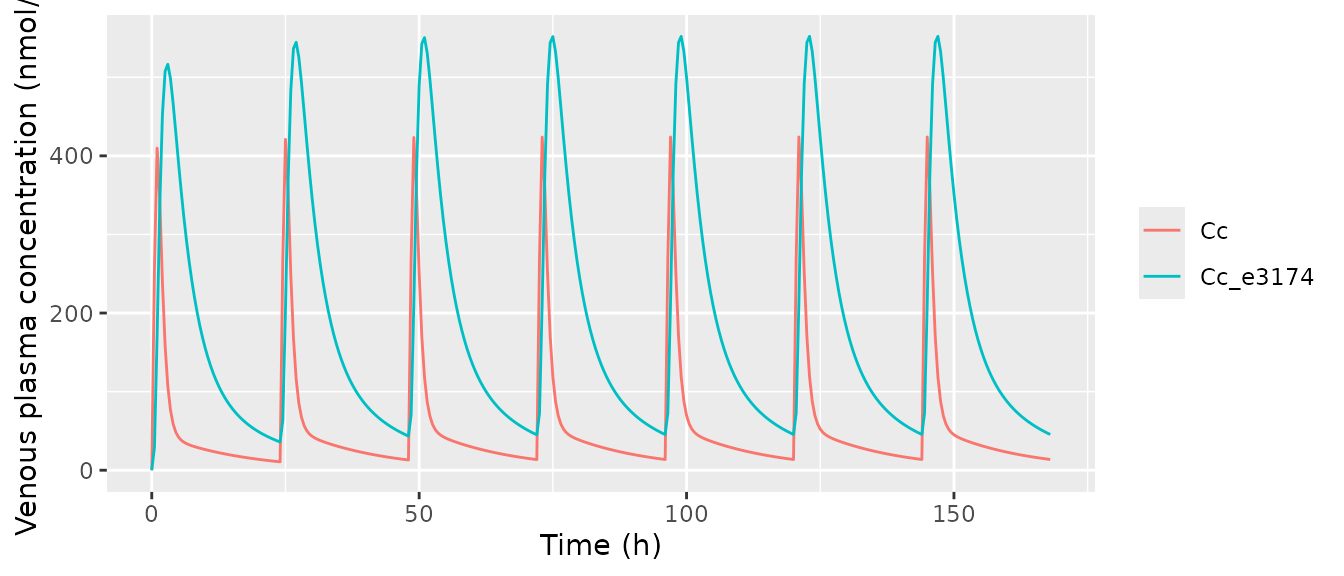
Non-compartmental analysis
PKNCA on single oral doses of 10, 25, 50 and 100 mg, for losartan and E3174.
nca_doses <- c(10, 25, 50, 100)
nca_sim <- bind_rows(lapply(seq_along(nca_doses), function(i) {
  sim_los(nca_doses[i], hours = 48, by_min = 10) |>
    mutate(id = i, treatment = paste(nca_doses[i], "mg"), dose = nca_doses[i])
}))

conc_long <- nca_sim |>
  select(id, treatment, hour, losartan = Cc, E3174 = Cc_e3174) |>
  pivot_longer(c(losartan, E3174), names_to = "analyte", values_to = "conc") |>
  filter(!is.na(conc)) |>
  mutate(conc = pmax(conc, 0) / 1000) # umol/L

dose_df <- nca_sim |>
  distinct(id, treatment, dose) |>
  mutate(hour = 0) |>
  as.data.frame()

o_conc <- PKNCA::PKNCAconc(as.data.frame(conc_long), conc ~ hour | treatment + id / analyte)
o_dose <- PKNCA::PKNCAdose(dose_df, dose ~ hour | treatment + id)
nca_res <- PKNCA::pk.nca(PKNCA::PKNCAdata(
  o_conc, o_dose,
  intervals = data.frame(start = 0, end = Inf, cmax = TRUE, tmax = TRUE,
                         aucinf.obs = TRUE, half.life = TRUE)
))

nca_tab <- as.data.frame(nca_res$result) |>
  filter(PPTESTCD %in% c("cmax", "tmax", "aucinf.obs", "half.life")) |>
  select(treatment, analyte, PPTESTCD, PPORRES) |>
  pivot_wider(names_from = PPTESTCD, values_from = PPORRES) |>
  arrange(analyte, as.numeric(sub(" mg", "", treatment)))
nca_tab |>
  rename("Dose" = treatment, "Analyte" = analyte, "Cmax (umol/L)" = cmax,
         "tmax (h)" = tmax, "AUCinf (umol*h/L)" = aucinf.obs,
         "Half-life (h)" = half.life) |>
knitr::kable(digits = 3)| Dose | Analyte | Cmax (umol/L) | tmax (h) | Half-life (h) | AUCinf (umol*h/L) |
|---|---|---|---|---|---|
| 10 mg | E3174 | 0.105 | 2.833 | 10.809 | 0.897 |
| 25 mg | E3174 | 0.258 | 2.833 | 10.811 | 2.236 |
| 50 mg | E3174 | 0.502 | 2.833 | 10.820 | 4.449 |
| 100 mg | E3174 | 0.946 | 3.000 | 10.835 | 8.793 |
| 10 mg | losartan | 0.075 | 1.000 | 10.960 | 0.258 |
| 25 mg | losartan | 0.192 | 1.000 | 10.954 | 0.659 |
| 50 mg | losartan | 0.401 | 1.000 | 10.954 | 1.366 |
| 100 mg | losartan | 0.876 | 1.000 | 10.956 | 2.946 |
Over 10-100 mg losartan AUCinf rises 11.4-fold and E3174 AUCinf 9.8-fold for a 10-fold dose increase (saturable CYP2C9 conversion), and the terminal half-life of about 11 h is the slow tail of a multi-phasic profile; Figure 3C plots half-lives of about 6.6-8.3 h, which the authors computed with their own terminal-phase window, so half-life is not compared. Figure 3C also plots AUC and Cmax against dose; the values read off that panel at 50 mg are compared below.
fig3c <- tibble::tribble(
  ~treatment, ~analyte, ~cmax, ~aucinf.obs,
  "50 mg", "losartan", 0.40, 1.3,
  "50 mg", "E3174", 0.50, 4.4
)
sim_50 <- as.data.frame(nca_res$result) |> filter(treatment == "50 mg")
nca_cmp <- nlmixr2lib::ncaComparisonTable(
  simulated = sim_50,
  reference = fig3c,
  by = c("treatment", "analyte"),
  params = c("cmax", "aucinf.obs"),
  units = c(cmax = "umol/L", aucinf.obs = "umol*h/L"),
  tolerance_pct = 20
)
knitr::kable(nca_cmp, caption = "Simulated NCA vs. Figure 3C of Tensil 2026 (read off the plot). * differs by >20%.")| NCA parameter | treatment | analyte | Reference | Simulated | % diff |
|---|---|---|---|---|---|
| Cmax (umol/L) | 50 mg | losartan | 0.4 | 0.401 | +0.2% |
| Cmax (umol/L) | 50 mg | E3174 | 0.5 | 0.502 | +0.5% |
| AUC0-∞ (obs) (umol*h/L) | 50 mg | losartan | 1.3 | 1.37 | +5.1% |
| AUC0-∞ (obs) (umol*h/L) | 50 mg | E3174 | 4.4 | 4.45 | +1.1% |
nca_50 <- nca_tab |> filter(treatment == "50 mg")
stopifnot(
  abs(nca_50$cmax[nca_50$analyte == "losartan"] / 0.40 - 1) < 0.1,
  abs(nca_50$cmax[nca_50$analyte == "E3174"] / 0.50 - 1) < 0.1,
  abs(nca_50$aucinf.obs[nca_50$analyte == "E3174"] / 4.4 - 1) < 0.1,
  # Losartan peaks within about 1 h and E3174 later (about 3 h), as in the
  # clinical data quoted in the Introduction (1-2 h and 3-4 h).
  nca_50$tmax[nca_50$analyte == "losartan"] <= 1.5,
  nca_50$tmax[nca_50$analyte == "E3174"] > 2, nca_50$tmax[nca_50$analyte == "E3174"] < 4
)
Oral bioavailability
po <- sim_los(50, hours = 96, by_min = 5)
iv <- sim_los(30, route = "depot_iv", hours = 96, by_min = 5)
f_oral <- (trap(po$hour, po$Cc) / 50) / (trap(iv$hour, iv$Cc) / 30)
f_oral
#> [1] 0.2935073
stopifnot(f_oral > 0.2, f_oral < 0.4)
The model’s oral bioavailability of losartan is about 29%, close to the approximately 33% quoted in the paper’s Introduction.
Assumptions and deviations / Errata
1. The model equations come from the authors’ SBML
archive. The paper and its supplement give the parameter values
but no rate law or ODE. The equations were taken from the authors’
archive at release 0.8.0, the release the paper cites; its parameters
match Supplementary Tables S2, S3 and S7. A later release (0.9.0)
re-fits several parameters (its release notes list, for example,
Kp_los 3.262 to 1.167 and E50_e3174 2.91e-4 to
2.07e-4 mmol/L) and is not the published model.
2. Table S3 prints the aldosterone secretion rate in the
wrong unit. Table S3 lists
ALDSEC_k = 1.011 mmole/min, Table S7 and the SBML give
1.01e-6 mmol/min. Because the aldosterone degradation constant is
ALDSEC_k / ald_ref, only the second value keeps aldosterone
at its 250 pmol/L baseline with the published dynamics, so 1.0105e-6
mmol/min is used.
3. Aldosterone secretion does not depend on angiotensin
II. Results 3.2 says “angiotensin II stimulates aldosterone
secretion”, but in the archived model aldosterone secretion is
ALDSEC_k * (1 - fe_e3174) and angiotensin II has no
downstream effect. The model is carried over as archived, so angiotensin
I and II are outputs only. Renin, too, responds only to E3174 (there is
no angiotensin-II feedback), and the renin turnover rate constant
(rensec_k / (ren_ref * vplasma), about 2e7 /min) makes
renin follow E3174 instantaneously.
4. Omitted states. The SBML carries seven further
states that never change the solution: three bile pools whose inflow and
outflow are the same expression (so they stay at zero; the biliary flux
goes straight to the gut lumen here), an unused stomach pool, the
constant angiotensinogen pool (here the parameter
anggen_ref), and two cumulative-infusion counters. An
intravenous infusion (SBML Ri_los, Ri_e3174)
is given here as an ordinary rate into
depot_iv or depot_iv_e3174, which is the same
input.
5. Units are rescaled. The SBML works in mmol and
mmol/L. Drug states here are in umol/L, the RAAS hormones in pmol/L and
the outputs Cc, Cc_e3174, Cc_l158
in nmol/L, with the Michaelis constant and E50 converted inside
model(). The rescaling is exact (the roadrunner comparison
above confirms it) and keeps baseline renin (1e-9 mmol/L) well above the
solver’s absolute tolerance.
6. Study-specific baselines. The per-study
simulations reset the baseline hormone levels and blood pressures to
each study’s values (Supplementary Table S5). These are the parameters
ren_ref, ang1_ref, ang2_ref,
ald_ref, sbp_ref and dbp_ref
(pmol/L and mmHg); override them with ini() to reproduce a
given study. The defaults are the model’s reference values (renin 1,
angiotensin I 10, angiotensin II 8, aldosterone 250 pmol/L; 120/80
mmHg).
7. Covariate encoding. Hepatic impairment is the
complement of the source’s cirrhosis severity
(HEPFUNC_REL = 1 - f_cirrhosis). The paper does not print a
genotype-to-activity map for CYP2C9 or ABCB1, nor a
KDIGO-to-renal-function map; the values used in each study simulation
are listed in Supplementary Table S5 and quoted above. ABCB1 activity is
kept as the parameter f_abcb1 because the library has no
continuous P-glycoprotein activity covariate.
8. Known model limitations reported by the authors. The model under-predicts E3174 accumulation in cirrhosis and over-predicts it in renal impairment relative to clinical data (Sections 3.4 and 3.5), and Figure 2 reports higher urinary recovery than the model produces. These are properties of the published model and are reproduced, not corrected.