Taspoglutide MBMA (Li 2015)
Source:vignettes/articles/Li_2015_taspoglutide_mbma.Rmd
Li_2015_taspoglutide_mbma.RmdModel and source
- Citation: Li HQ, Xu JY, Jin L, Xin JL. Utilization of model-based meta-analysis to delineate the net efficacy of taspoglutide from the response of placebo in clinical trials. Saudi Pharm J. 2015 Jul;23(3):241-249. doi:10.1016/j.jsps.2014.11.008.
- Description: see
rxode2::rxode(readModelDb("Li_2015_taspoglutide_mbma"))$description. - Article (open access, CC BY-NC-ND): https://doi.org/10.1016/j.jsps.2014.11.008
Li et al. (2015) performed a model-based meta-analysis (MBMA) of nine published phase-2 / phase-3 trials of taspoglutide (a long-acting human GLP-1 receptor agonist, given as once-weekly subcutaneous injection in type 2 diabetes). Eight trials (3,702 patients) were pooled for model development; the ninth (Rosenstock 2013 T-emerge 4, 797 patients) was held out for external validation. The authors digitised mean change-from-baseline trajectories for fasting plasma glucose (FPG) and glycosylated hemoglobin (HbA1c) over 8-52 week treatment durations and fitted two coupled PD models in Monolix 4.2/4.3 (SAEM).
Each endpoint is the sum of a placebo response and a drug response, both following an exponential approach to an asymptote (Li 2015 Eq. 1-2). The FPG drug asymptote is an Emax saturation in taspoglutide concentration; the HbA1c drug asymptote is an Emax saturation in the drug-induced FPG reduction (a sequential PD cascade: drug -> FPG -> HbA1c).
Population
The model was fitted on study-arm-mean data pooled across 8 trials in
adults with type 2 diabetes (3,702 patients; treatment durations 8-52
weeks). The trials cover monotherapy and combination regimens
(drug-naive; inadequately controlled on metformin; failing metformin +
sulphonylurea; metformin + TZD; etc.; Li 2015 Table 1). Per-trial
baseline demographics are not pooled in the paper. See the model’s
population metadata
(readModelDb("Li_2015_taspoglutide_mbma")$population) for
the per-trial patient counts and dosing regimens.
Scope. The model is calibrated and intended for study-arm-mean PD simulation (each simulated “subject” represents a trial arm). It is not suitable for individual-subject simulation – the between-trial random effects do not encode within-trial between-subject variability.
Source trace
Per-parameter origin is recorded as in-file comments next to every
ini() entry in
inst/modeldb/specificDrugs/Li_2015_taspoglutide_mbma.R. The
table below collects them in one place.
| Equation / parameter | Value | Source location |
|---|---|---|
FPG placebo response:
d(fpg_placebo)/dt = Kp_F (Pmax_F - fpg_placebo)
|
n/a | Li 2015 Eq. 1 |
FPG drug response:
d(fpg_drug)/dt = Kdrug_F (Dmax_F * C / (IC50_F + C) - fpg_drug)
|
n/a | Li 2015 Eq. 2 |
Pmax_F (mmol/L) |
-0.371 | Li 2015 Table 2 (fixed; placebo-only fit, ITV 29.8%) |
Kp_F (1/week) |
0.781 | Li 2015 Table 2 (fixed; placebo-only fit, ITV 37.8%) |
Dmax_F (mmol/L) |
-2.39 | Li 2015 Table 2 (RSE 6%, ITV 24.8%) |
IC50_F (pmol/L) |
25.3 | Li 2015 Table 2 (RSE 0%; ITV 5.43%) |
Kdrug_F (1/week) |
2.0 | Li 2015 Table 2 (RSE 2%, ITV 12.5%) |
b (FPG residual) |
0.194 | Li 2015 Table 2 (RSE 8%) |
c (FPG residual power, not encoded) |
0.182 | Li 2015 Table 2 (RSE 37%) |
HbA1c placebo response: same form as FPG with Pmax_Hb,
Kp_Hb
|
n/a | Li 2015 Eq. 1 |
HbA1c drug response:
d(hba1c_drug)/dt = Kdrug_Hb (Dmax_Hb * fpg_drug / (IC50_Hb + fpg_drug) - hba1c_drug)
|
n/a | Li 2015 Eq. 2; Section 3.2 (metric is FPG change) |
Pmax_Hb (%) |
-0.253 | Li 2015 Table 3 (fixed; placebo-only fit, ITV 15.2%) |
Kp_Hb (1/week) |
0.382 | Li 2015 Table 3 (fixed; placebo-only fit, ITV 14.7%) |
Dmax_Hb (%) |
-1.74 | Li 2015 Table 3 (RSE 8%, ITV 8.65%) |
IC50_Hb (mmol/L) |
-1.81 | Li 2015 Table 3 (RSE 15%, ITV 26.8%) |
Kdrug_Hb (1/week) |
0.249 | Li 2015 Table 3 (RSE 13%, ITV 19.9%) |
a (HbA1c residual additive) |
0.00532 | Li 2015 Table 3 (RSE 16%) |
b (HbA1c residual proportional) |
0.0717 | Li 2015 Table 3 (RSE 13%) |
c (HbA1c residual power, not encoded) |
0.239 | Li 2015 Table 3 (RSE 66%) |
| Drug exposure metric (Cavg w2-w4): 0 / 59.85 / 119.7 pmol/L for placebo / 10 mg / 20 mg QW | n/a | Li 2015 Section 3.2 |
Simulation
The model accepts a single MBMA covariate,
METRIC_TASPO_C – the study-arm average plasma taspoglutide
concentration between weeks 2 and 4 (pmol/L). Supplied values: 0
(placebo), 59.85 (10 mg QW), 119.7 (20 mg QW). There are no drug-dose
events; the metric is the only driver of the drug arm.
mod         <- readModelDb("Li_2015_taspoglutide_mbma")
mod_typical <- mod |> rxode2::zeroRe()
#> ℹ parameter labels from comments will be replaced by 'label()'

times <- seq(0, 52, by = 0.5)

make_arm <- function(metric_c, label, id) {
  data.frame(
    id             = id,
    time           = times,
    evid           = 0L,
    amt            = NA_real_,
    cmt            = "FPG",
    METRIC_TASPO_C = metric_c,
    arm            = label,
    stringsAsFactors = FALSE
  )
}

typical_events <- rbind(
  make_arm(0,     "Placebo",         1L),
  make_arm(59.85, "Taspoglutide 10 mg QW", 2L),
  make_arm(119.7, "Taspoglutide 20 mg QW", 3L)
)
stopifnot(!anyDuplicated(typical_events[, c("id", "time", "evid")]))

sim_typical <- as.data.frame(
  rxode2::rxSolve(
    mod_typical,
    events = typical_events,
    keep   = c("arm", "METRIC_TASPO_C"),
    addDosing = FALSE
  )
)
#> ℹ omega/sigma items treated as zero: 'eta_study_pmax_f', 'eta_study_lkp_f', 'eta_study_dmax_f', 'eta_study_ic50_f', 'eta_study_lkdrug_f', 'eta_study_pmax_hb', 'eta_study_lkp_hb', 'eta_study_dmax_hb', 'eta_study_ic50_hb', 'eta_study_lkdrug_hb'
#> Warning: multi-subject simulation without without 'omega'
Asymptote sanity check
For a sustained constant metric C, the FPG asymptote is
Pmax_F + Dmax_F * C / (IC50_F + C) and the HbA1c asymptote
is
Pmax_Hb + Dmax_Hb * fpg_drug_asymp / (IC50_Hb + fpg_drug_asymp).
These algebraic values must match the simulated trajectory at large
t.
pmax_f  <- -0.371; dmax_f <- -2.39; ic50_f <- 25.3
pmax_hb <- -0.253; dmax_hb <- -1.74; ic50_hb <- -1.81

closed_form <- function(C) {
  fpg_drug_asymp <- dmax_f * C / (ic50_f + C)
  fpg_asymp      <- pmax_f + fpg_drug_asymp
  hba1c_drug_asymp <- if (C == 0) 0 else dmax_hb * fpg_drug_asymp / (ic50_hb + fpg_drug_asymp)
  hba1c_asymp    <- pmax_hb + hba1c_drug_asymp
  c(FPG_asymp = fpg_asymp, HbA1c_asymp = hba1c_asymp)
}

closed <- rbind(
  Placebo                = closed_form(0),
  `Taspoglutide 10 mg QW` = closed_form(59.85),
  `Taspoglutide 20 mg QW` = closed_form(119.7)
)
sim_endpoint <- sim_typical |>
  dplyr::filter(time == 52) |>
  dplyr::select(arm, FPG, HbA1c)

compare <- data.frame(
  arm        = rownames(closed),
  FPG_closed = round(closed[, "FPG_asymp"],   3),
  FPG_sim    = round(sim_endpoint$FPG[match(rownames(closed), sim_endpoint$arm)],   3),
  HbA1c_closed = round(closed[, "HbA1c_asymp"], 3),
  HbA1c_sim    = round(sim_endpoint$HbA1c[match(rownames(closed), sim_endpoint$arm)], 3),
  row.names = NULL
)
knitr::kable(compare,
caption = "Closed-form vs simulated asymptote at week 52 (typical values).")| arm | FPG_closed | FPG_sim | HbA1c_closed | HbA1c_sim |
|---|---|---|---|---|
| Placebo | -0.371 | -0.371 | -0.253 | -0.253 |
| Taspoglutide 10 mg QW | -2.051 | -2.051 | -1.091 | -1.091 |
| Taspoglutide 20 mg QW | -2.344 | -2.344 | -1.160 | -1.160 |
The simulated and closed-form values must agree to ~3 decimals; a mismatch would indicate an ODE-encoding error.
Half-life sanity check
For an exponential approach
d(state)/dt = k * (asymp - state), the time to
half-asymptote is ln(2)/k.
half_life <- data.frame(
  parameter        = c("Kp_F", "Kdrug_F", "Kp_Hb", "Kdrug_Hb"),
  rate_per_week    = c(0.781, 2.0, 0.382, 0.249),
  half_life_weeks  = round(log(2) / c(0.781, 2.0, 0.382, 0.249), 3),
  half_life_days   = round(7 * log(2) / c(0.781, 2.0, 0.382, 0.249), 2),
  paper_reports    = c(
    "placebo FPG half-life not given numerically",
    "kdrug_F = 2.0/week -> half-life 2.4 days (paper Section 3.4)",
    "placebo HbA1c half-life not given numerically",
    "kdrug_Hb = 0.249/week -> half-life 2.8 weeks (paper Section 3.4)"
  )
)
knitr::kable(half_life,
caption = "Drug-effect time-to-half-asymptote: simulated vs paper text.")| parameter | rate_per_week | half_life_weeks | half_life_days | paper_reports |
|---|---|---|---|---|
| Kp_F | 0.781 | 0.888 | 6.21 | placebo FPG half-life not given numerically |
| Kdrug_F | 2.000 | 0.347 | 2.43 | kdrug_F = 2.0/week -> half-life 2.4 days (paper Section 3.4) |
| Kp_Hb | 0.382 | 1.815 | 12.70 | placebo HbA1c half-life not given numerically |
| Kdrug_Hb | 0.249 | 2.784 | 19.49 | kdrug_Hb = 0.249/week -> half-life 2.8 weeks (paper Section 3.4) |
Replicate published figures
Figure 1 – FPG response over time
fpg_plot <- sim_typical |>
  dplyr::select(time, arm, FPG, fpg_placebo, fpg_drug) |>
  tidyr::pivot_longer(c(FPG, fpg_placebo, fpg_drug),
                      names_to = "component", values_to = "delta_FPG") |>
  dplyr::mutate(component = factor(component,
                                   levels = c("FPG", "fpg_placebo", "fpg_drug"),
                                   labels = c("Total FPG response",
                                              "Placebo component",
                                              "Drug component")))

ggplot(fpg_plot |> dplyr::filter(component == "Total FPG response"),
       aes(time, delta_FPG, colour = arm)) +
  geom_line(linewidth = 1) +
  facet_wrap(~ arm, ncol = 3) +
  labs(x = "Time (weeks)",
       y = "FPG change from baseline (mmol/L)",
       title = "Figure 1 - FPG change-from-baseline over time",
       caption = "Replicates Figure 1 of Li 2015 (panel A: placebo; panel B: drug response).") +
  theme_minimal() +
  theme(legend.position = "none")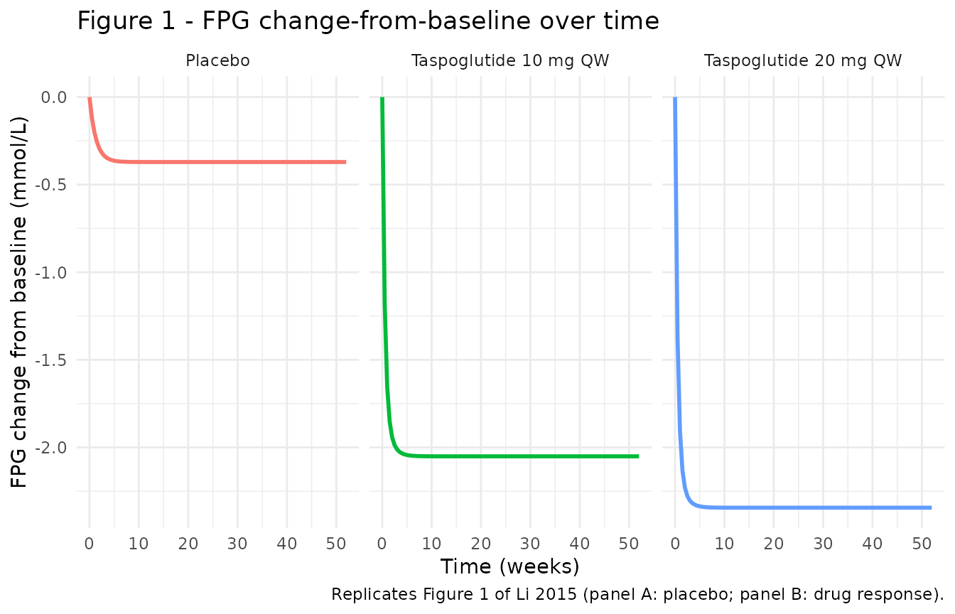
The paper’s Figure 1A (placebo, single arm) shows a slow FPG decline to about -0.4 mmol/L by week 4-6 and a sustained plateau; Figure 1B (drug response, pooled across 10 and 20 mg) shows a rapid drop to about -2.1 / -2.3 mmol/L within 4-6 weeks and a sustained plateau. The simulated trajectories above match those asymptotes (placebo -0.37, 10 mg -2.05, 20 mg -2.34 mmol/L) and the drug-effect 2-3 day half-life.
Figure 2 – HbA1c response over time
hba1c_plot <- sim_typical |>
  dplyr::select(time, arm, HbA1c, hba1c_placebo, hba1c_drug)

ggplot(hba1c_plot, aes(time, HbA1c, colour = arm)) +
  geom_line(linewidth = 1) +
  facet_wrap(~ arm, ncol = 3) +
  labs(x = "Time (weeks)",
       y = "HbA1c change from baseline (%)",
       title = "Figure 2 - HbA1c change-from-baseline over time",
       caption = "Replicates Figure 2 of Li 2015 (panel A: placebo; panel B: drug response).") +
  theme_minimal() +
  theme(legend.position = "none")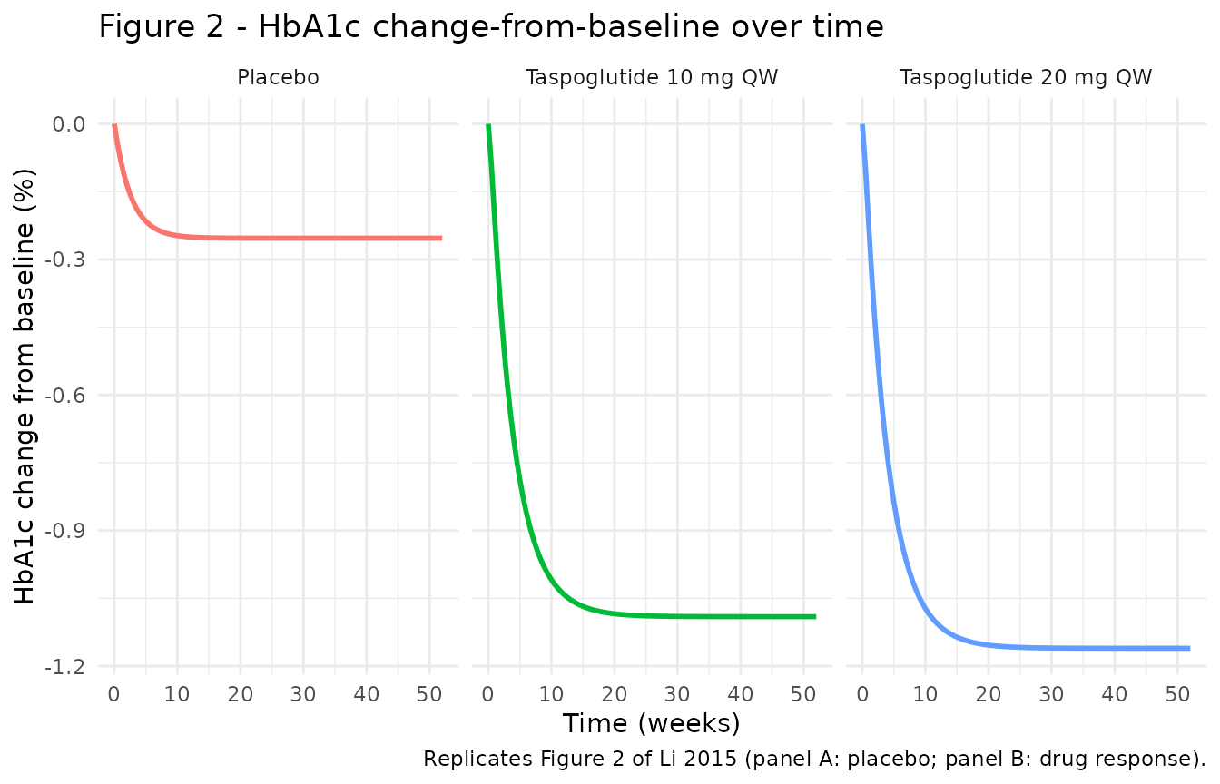
Li 2015 Figure 2A (placebo) reaches about -0.25% within ~5-10 weeks; Figure 2B (drug response) reaches about -1.0 to -1.2% by ~20-25 weeks at both doses (Section 3.4: “the responses between dose 10 and 20 mg did not show significant differences in the reduction of HbA1c”). The simulated trajectories above reach -0.25% (placebo), -1.09% (10 mg) and -1.16% (20 mg). The 2.8-week drug-effect half-life means steady state is reached around week ~14 (5 half-lives).
Variability – between-trial scope
The model encodes between-trial variability (ITV) as study-level etas (one per parameter; diagonal). Stochastic simulation gives the variability across trial-mean trajectories – not across individual patients within a trial.
set.seed(20251029)

n_trials_per_arm <- 200L

vpc_arms <- list(
  list(metric = 0,     label = "Placebo"),
  list(metric = 59.85, label = "Taspoglutide 10 mg QW"),
  list(metric = 119.7, label = "Taspoglutide 20 mg QW")
)

vpc_events <- do.call(rbind, lapply(seq_along(vpc_arms), function(k) {
  arm <- vpc_arms[[k]]
  id_offset <- (k - 1L) * n_trials_per_arm
  do.call(rbind, lapply(seq_len(n_trials_per_arm), function(i) {
    make_arm(arm$metric, arm$label, id = id_offset + i)
  }))
}))
stopifnot(!anyDuplicated(vpc_events[, c("id", "time", "evid")]))

sim_vpc <- as.data.frame(
  rxode2::rxSolve(
    mod,
    events = vpc_events,
    keep   = c("arm", "METRIC_TASPO_C"),
    addDosing = FALSE,
    nStud  = 1L
  )
)
#> ℹ parameter labels from comments will be replaced by 'label()'

vpc_summary <- sim_vpc |>
  dplyr::group_by(arm, time) |>
  dplyr::summarise(
    FPG_q05   = quantile(FPG,   0.05, na.rm = TRUE),
    FPG_q50   = quantile(FPG,   0.50, na.rm = TRUE),
    FPG_q95   = quantile(FPG,   0.95, na.rm = TRUE),
    HbA1c_q05 = quantile(HbA1c, 0.05, na.rm = TRUE),
    HbA1c_q50 = quantile(HbA1c, 0.50, na.rm = TRUE),
    HbA1c_q95 = quantile(HbA1c, 0.95, na.rm = TRUE),
    .groups   = "drop"
  )

ggplot(vpc_summary, aes(time)) +
  geom_ribbon(aes(ymin = FPG_q05, ymax = FPG_q95, fill = arm), alpha = 0.25) +
  geom_line(aes(y = FPG_q50, colour = arm), linewidth = 1) +
  facet_wrap(~ arm, ncol = 3) +
  labs(x = "Time (weeks)",
       y = "FPG change from baseline (mmol/L)",
       title = "Between-trial 5-50-95% intervals for FPG",
       caption = "n = 200 simulated trial-mean trajectories per arm.") +
  theme_minimal() +
  theme(legend.position = "none")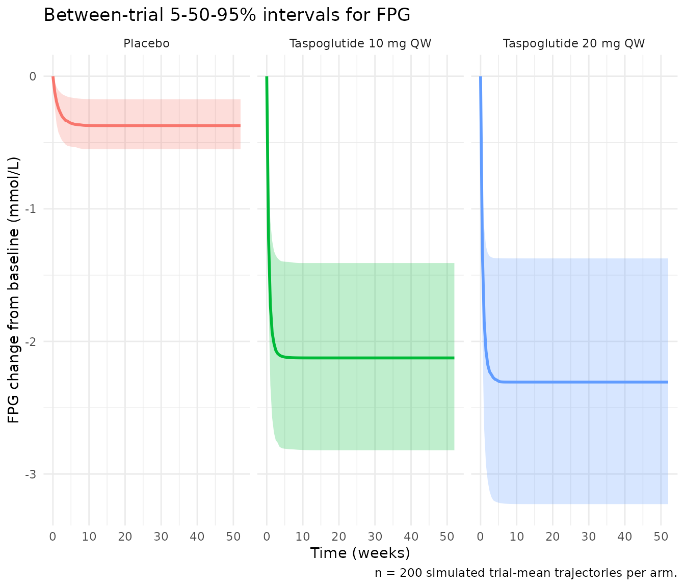
ggplot(vpc_summary, aes(time)) +
  geom_ribbon(aes(ymin = HbA1c_q05, ymax = HbA1c_q95, fill = arm), alpha = 0.25) +
  geom_line(aes(y = HbA1c_q50, colour = arm), linewidth = 1) +
  facet_wrap(~ arm, ncol = 3) +
  labs(x = "Time (weeks)",
       y = "HbA1c change from baseline (%)",
       title = "Between-trial 5-50-95% intervals for HbA1c",
       caption = "n = 200 simulated trial-mean trajectories per arm.") +
  theme_minimal() +
  theme(legend.position = "none")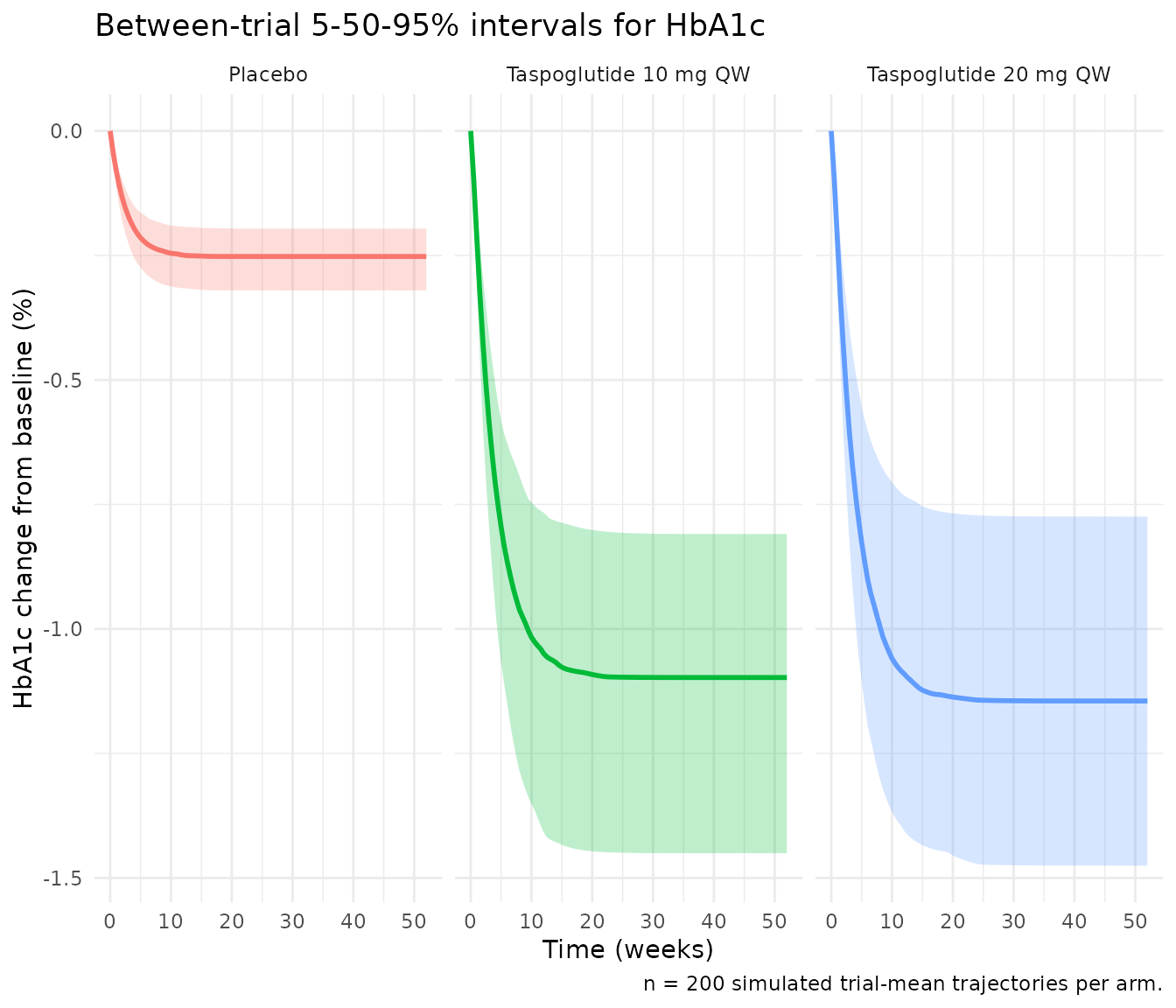
Assumptions and deviations
Multi-output PD model, no PKNCA validation. Taspoglutide concentration enters this MBMA model as a fixed scalar covariate (study-arm Cavg weeks 2-4), not as a simulated PK profile. There are no dose events and no AUC / Cmax / half-life PK metrics to compute via PKNCA. Validation follows the endogenous-model style: closed-form asymptote check (Eq. 2), rate-of-approach half-life check, and per-arm trajectory comparison to Figures 1 and 2.
Compartment naming. The four ODE states (
fpg_placebo,fpg_drug,hba1c_placebo,hba1c_drug) are paper-meaningful PD compartments rather than canonical PK names (central,peripheral1, etc.). The model is a meta-analytic PD model with no concentration-versus-time PK profile. The multi-output PD nature is in line withChoy_2016_T2DM_WHIG.R(FPG, FSI, HbA1c, WGT) but with the dose-response coupling Li 2015 reports rather than the homeostatic feedback Choy 2016 uses.Eta naming –
eta_study_<param>. Between-trial random effects are namedeta_study_pmax_fetc. to make the MBMA scope explicit (per the skill’s MBMA guidance, “Encode between-study variance as a study-level eta … clearly labelled to distinguish from the popPK pattern”). The lint flags these as “no matching fixed-effect parameter_study_pmax_f” – the pairing iseta_study_pmax_f<->pmax_f, but the lint’s regex only understands theeta<param>pattern. The deviation is intentional.METRIC_TASPO_Ccovariate not in canonical register. The canonical covariate-columns register tracks individual-level pop-PK covariates; MBMA study-arm-level drug-exposure columns are documented inline incovariateDataper the precedent set byVargo_2014_statins_ezetimibe_mbma.R.-
ITV reading. The paper reports inter-trial variability as percentages in Tables 2 and 3 without stating whether the column is the SD of the random effect, the relative SD (SD/typical), or a derived CV%. The implementation reads:
- For the exponential model (Kp, Kdrug): ITV(%) is approximate CV%, so
omega^2 = log((ITV/100)^2 + 1). - For the additive model (Pmax, Dmax, IC50): ITV(%) is the SD divided
by the absolute typical value times 100, so
omega = (ITV/100) * |P_pop|andomega^2 = ((ITV/100) * |P_pop|)^2. These are the most common Monolix-output conventions; the alternative reading (omega itself as a percent) would scale the ITV variances by an approximately constant factor and would shift the VPC prediction-interval width but not the typical trajectory. The Section 2.6 prose specifies the exponential and additive distributional forms but not the column units.
- For the exponential model (Kp, Kdrug): ITV(%) is approximate CV%, so
Power-error simplification (
cnot encoded). Li 2015 Tables 2 and 3 listbandcfor the FPG residual anda,b,cfor the HbA1c residual. The text Eq. 5 simplifies the FPG error toY = F + b*F*epsand Eq. 6 the HbA1c error toY = F + (a + b*F^c)*eps. The table is canonical (the Eq. 5 prose appears incomplete relative to the table). nlmixr2 has no clean power-of-prediction residual syntax, so the implementation usesprop(propSd)on FPG withpropSd_FPG = b = 0.194andadd(addSd) + prop(propSd)on HbA1c withaddSd_HbA1c = a = 0.00532andpropSd_HbA1c = b = 0.0717. Thecpower exponent (0.182 for FPG, 0.239 for HbA1c) is omitted; in practice this affects the residual-error scale at endpoint magnitudes far from |F| ~ 1 only modestly.HbA1c metric uses simulated
fpg_drugonly, not population-prediction FPG. Li 2015 Section 3.2 specifies that the HbA1c metric is “the population prediction values for taspoglutide 10 and 20 mg in FPG modeling”. The implementation uses the current trial’sfpg_drugstate (the drug-induced FPG reduction) as the HbA1c metric, which equals the population prediction in the typical-value simulation (rxode2::zeroRe(mod)). When ITV is active, this propagates the FPG ITV through the HbA1c Emax – a small extra source of HbA1c trial-mean variability that the paper’s two-stage fitting procedure avoided. For point predictions (typical values) the two procedures agree exactly.No erratum found. PubMed and the journal landing page for doi:10.1016/j.jsps.2014.11.008 were checked at extraction time; no errata or author corrections are noted.