Remimazolam tosilate (HR7056) sedation PK/PD (Zhou 2018)
Source:vignettes/articles/Zhou_2018_remimazolam.Rmd
Zhou_2018_remimazolam.RmdModel and source
Zhou 2018 reports a single-ascending-dose study of the benzodiazepine sedative remimazolam tosilate (development code HR7056) in Chinese healthy volunteers, and fits three models to it. The paper is explicit that the analysis was two-stage rather than joint: “we did not make attempts to model the PKs and PDs concurrently because the quality of the kinetic data was so reliable that a two-stage approach was used. Firstly, the pharmacokinetic parameters for each subject were estimated, using the final PK compartmental model, which was then used to simulate arterial concentration profiles for the pharmacodynamic modeling.”
Three model files follow that structure, and all three point at this vignette.
- Article: https://doi.org/10.3389/fphar.2018.01316 (open access, CC BY; PMC6252322)
- Trial registration: NCT01970072
pk <- rxode2::rxode(readModelDb("Zhou_2018_remimazolam"))
#> ℹ parameter labels from comments will be replaced by 'label()'
bis <- rxode2::rxode(readModelDb("Zhou_2018_remimazolam_bis"))
#> ℹ parameter labels from comments will be replaced by 'label()'
moaas <- rxode2::rxode(readModelDb("Zhou_2018_remimazolam_moaas"))
#> ℹ parameter labels from comments will be replaced by 'label()'

tibble::tibble(
  Model = c(
    "Zhou_2018_remimazolam",
    "Zhou_2018_remimazolam_bis",
    "Zhou_2018_remimazolam_moaas"
  ),
  Role = c(
    "Three-compartment arterial-plasma popPK (Table 1)",
    "Effect-compartment sigmoid Imax model on the Bispectral Index (Table 2, FINAL BIS MODEL)",
    "Effect-compartment ordered-categorical model on the MOAA/S score (Table 2, FINAL MOAA/S MODEL)"
  ),
  Software = c("Phoenix NLME 1.2 (FOCE-I)", "Phoenix NLME 1.2", "NONMEM 7.2 (conditional Laplacian)")
) |>
knitr::kable(caption = "The three models Zhou 2018 fits, and where each one's estimates live.")| Model | Role | Software |
|---|---|---|
| Zhou_2018_remimazolam | Three-compartment arterial-plasma popPK (Table 1) | Phoenix NLME 1.2 (FOCE-I) |
| Zhou_2018_remimazolam_bis | Effect-compartment sigmoid Imax model on the Bispectral Index (Table 2, FINAL BIS MODEL) | Phoenix NLME 1.2 |
| Zhou_2018_remimazolam_moaas | Effect-compartment ordered-categorical model on the MOAA/S score (Table 2, FINAL MOAA/S MODEL) | NONMEM 7.2 (conditional Laplacian) |
- Citation: Zhou Y, Hu P, Huang Y, Nuoer S, Song K, Wang H, Wen J, Jiang J, Chen X. Population Pharmacokinetic/Pharmacodynamic Model-Guided Dosing Optimization of a Novel Sedative HR7056 in Chinese Healthy Subjects. Front Pharmacol. 2018;9:1316. doi:10.3389/fphar.2018.01316. PMC6252322.
Population
Sixty-three Chinese healthy volunteers received HR7056 as a single 1-minute intravenous injection across 11 ascending-dose cohorts spanning 0.01 to 0.45 mg/kg; a further 16 subjects received midazolam as an active comparator and are not part of any of these models. Fifty-one subjects were male and twelve female. Median (min-max) demographics were age 27 years (18-44), weight 63.8 kg (52.8-83.8) and height 169 cm (156-184). Eligibility required age 18-55 years, weight 50-100 kg and BMI 18-26 kg/m^2, which is why the authors attribute the complete absence of covariate effects to the narrowness of the cohort rather than to a genuine absence of covariate relationships.
The analysis dataset comprised 1197 arterial plasma concentrations, 1197 BIS values and 1197 MOAA/S scores. Arterial plasma - not venous - was sampled, which is why the paper labels V1 a “central (arterial) volume”; concentrations were assayed by UPLC-MS/MS validated over 0.5-1000 ng/mL.
The same information is available programmatically via each model’s
population metadata
(rxode2::rxode(readModelDb("Zhou_2018_remimazolam"))$population).
The MOAA/S scale (Zhou 2018 Table S1) runs from 5 down to 0. Note that a higher score means a more alert subject, so the drug drives the score down:
tibble::tibble(
  Score = 5:0,
  Responsiveness = c(
    "Fully alert; responds readily to name spoken in normal tone",
    "Lethargic response to name spoken in normal tone",
    "Responds only after name is called loudly and/or repeatedly",
    "Responds only after mild prodding or shaking",
    "Responds only after painful trapezius squeeze",
    "Does not respond to painful trapezius squeeze"
  )
) |>
knitr::kable(caption = "MOAA/S scoring standard (Zhou 2018 Table S1).")| Score | Responsiveness |
|---|---|
| 5 | Fully alert; responds readily to name spoken in normal tone |
| 4 | Lethargic response to name spoken in normal tone |
| 3 | Responds only after name is called loudly and/or repeatedly |
| 2 | Responds only after mild prodding or shaking |
| 1 | Responds only after painful trapezius squeeze |
| 0 | Does not respond to painful trapezius squeeze |
Source trace
Each ini() entry in the three model files carries an
in-file comment naming its source location. The table below collects
them.
| Model | Equation / parameter | Value | Source location |
|---|---|---|---|
| all three |
d/dt(central), d/dt(peripheral1),
d/dt(peripheral2)
|
n/a | Methods, Population Pharmacokinetic Modeling (“A three-compartment model was developed and these were expressed as clearances and volumes”) |
| all three |
lvc (V1) |
2.11 L | Table 1, Central (arterial) volume (RSE 4.0%, 95% CI 1.94-2.27) |
| all three |
lcl (CL) |
1.49 L/min | Table 1, Elimination clearance (RSE 1.9%, 95% CI 1.44-1.55) |
| all three |
lvp (V2) |
10.5 L | Table 1, Peripheral volume V2 (RSE 3.9%, 95% CI 9.73-11.3) |
| all three |
lq (Cl2) |
0.96 L/min | Table 1, Inter-compartmental clearance Cl2 (RSE 3.7%, 95% CI 0.89-1.03) |
| all three |
lvp2 (V3) |
22.7 L | Table 1, Peripheral volume V3 (RSE 4.1%, 95% CI 20.9-24.6) |
| all three |
lq2 (Cl3) |
0.27 L/min | Table 1, Inter-compartmental clearance Cl3 (RSE 4.0%, 95% CI 0.250-0.295) |
| all three |
etalvc, etalcl, etalvp,
etalq, etalvp2, etalq2
|
14.0, 11.5, 12.2, 13.3, 25.3, 18.7 % | Table 1, IIV% column; variance = (IIV%/100)^2 per the Methods definition of omega |
| PK | propSd |
0.138 | Table 1, sigma (RSE 2.9%); Results restate it as “residual variability was 13.8%” |
| BIS, MOAA/S | d/dt(effect) <- ke0 * (Cc - effect) |
n/a | Methods, Population Pharmacodynamic Modeling: dCe/dt = keo * (Cp - Ce) |
| BIS | BIS <- rbase - imax * effect^hill / (ec50^hill + effect^hill) |
n/a | Methods, Population Pharmacodynamic Modeling: E = E0 - IMax * Ce^gamma / (IC50^gamma + Ce^gamma) |
| BIS | lke0 |
0.0855 /min | Table 2, FINAL BIS MODEL, Ke0 (RSE 7.4%) |
| BIS | lec50 |
503 ng/mL | Table 2, FINAL BIS MODEL, IC50 (RSE 10.3%) |
| BIS | lhill |
1.50 | Table 2, FINAL BIS MODEL, Hill coefficient (RSE 7.8%) |
| BIS |
lrbase (E0) |
95.3 | Table 2, FINAL BIS MODEL, E0 (RSE 0.4%) |
| BIS | limax |
47.9 | Table 2, FINAL BIS MODEL, Imax (RSE 7.4%) |
| BIS |
etalke0, etalec50, etalhill,
etalrbase, etalimax
|
51.2, 41.1, 86.4, 1.56, 15.6 % | Table 2, FINAL BIS MODEL, IIV column |
| BIS |
propSd_BIS, addSd_BIS
|
0.0653 | Table 2, FINAL BIS MODEL, sigma (RSE 2.2%) - see Assumptions |
| MOAA/S |
Logit(x) = Baseline(x) + Imax * Ce^gamma / (IC50^gamma + Ce^gamma);
P(x) = 1/(1 + exp(-Logit(x)))
|
n/a | Methods, Population Pharmacodynamic Modeling (cumulative-logit and logistic-transform equations) |
| MOAA/S |
b1 … b5
|
-8.52, -2.44, -1.30, -1.15, -0.895 | Table 2, FINAL MOAA/S MODEL, rows B1-B5 |
| MOAA/S | lke0 |
0.05 /min | Table 2, FINAL MOAA/S MODEL, Ke0 (RSE 7.3%) |
| MOAA/S | lec50 |
436 ng/mL | Table 2, FINAL MOAA/S MODEL, IC50 (RSE 15.6%) |
| MOAA/S | lhill |
1.50 | Table 2, FINAL MOAA/S MODEL, Hill coefficient (RSE 14.6%) |
| MOAA/S | limax |
27.9 | Table 2, FINAL MOAA/S MODEL, Imax (RSE 9.4%) |
| MOAA/S |
etalke0, etalec50, etalhill,
etalimax
|
38.3, 45.5, 55.6, 17.6 % | Table 2, FINAL MOAA/S MODEL, IIV column |
| MOAA/S | addSd_prob_moaas_le1 |
0.05 | Not from the paper - placeholder; see Assumptions |
A closed-form check of the disposition model before anything else
The three-compartment system has an exact triexponential solution after an intravenous bolus. Reproducing it to solver precision confirms both that the micro-constants were derived correctly from the published clearances and volumes and that rxode2 is integrating the declared ODEs rather than silently substituting an auto-generated linear solution.
# Typical-value parameters, Zhou 2018 Table 1.
cl <- 1.49
vc <- 2.11
q <- 0.96
vp <- 10.5
q2 <- 0.27
vp2 <- 22.7

k10 <- cl / vc
k12 <- q / vc
k21 <- q / vp
k13 <- q2 / vc
k31 <- q2 / vp2

# Characteristic polynomial of the three-compartment system.
a2 <- k10 + k12 + k21 + k13 + k31
a1 <- k10 * k21 + k10 * k31 + k21 * k31 + k12 * k31 + k13 * k21
a0 <- k10 * k21 * k31
lambda <- sort(-Re(polyroot(c(a0, a1, a2, 1))), decreasing = TRUE)

coefA <- (k21 - lambda[1]) * (k31 - lambda[1]) /
  ((lambda[2] - lambda[1]) * (lambda[3] - lambda[1])) / vc
coefB <- (k21 - lambda[2]) * (k31 - lambda[2]) /
  ((lambda[1] - lambda[2]) * (lambda[3] - lambda[2])) / vc
coefC <- (k21 - lambda[3]) * (k31 - lambda[3]) /
  ((lambda[1] - lambda[3]) * (lambda[2] - lambda[3])) / vc

# ng/mL per mg of bolus dose.
cc_closed_form <- function(tt, dose) {
  dose * (coefA * exp(-lambda[1] * tt) + coefB * exp(-lambda[2] * tt) +
    coefC * exp(-lambda[3] * tt)) * 1000
}

half_lives <- log(2) / lambda
tibble::tibble(
  Phase = c("alpha", "beta", "gamma (terminal)"),
  `Rate constant (1/min)` = lambda,
  `Half-life (min)` = half_lives
) |>
knitr::kable(digits = 4, caption = "Hybrid rate constants of the Zhou 2018 disposition model.")| Phase | Rate constant (1/min) | Half-life (min) |
|---|---|---|
| alpha | 1.3240 | 0.5235 |
| beta | 0.0585 | 11.8488 |
| gamma (terminal) | 0.0099 | 69.9109 |
dose_mg <- 0.2 * 63.8 # 0.2 mg/kg at the cohort median weight
ev_bolus <- rxode2::et(amt = dose_mg, cmt = "central") |>
  rxode2::et(seq(0, 480, by = 0.25), cmt = "central")

sim_bolus <- rxode2::rxSolve(
  rxode2::zeroRe(pk), ev_bolus,
  returnType = "data.frame", atol = 1e-12, rtol = 1e-12
)
#> ℹ omega/sigma items treated as zero: 'etalvc', 'etalcl', 'etalvp', 'etalq', 'etalvp2', 'etalq2'

cf <- cc_closed_form(sim_bolus$time, dose_mg)
max_rel_ode <- max(abs(sim_bolus$Cc - cf) / pmax(cf, 1e-12))

# Exact AUC from zero to infinity of the triexponential, and the
# dose-recovery identity CL * AUCinf = Dose.
auc_inf_closed <- dose_mg * sum(c(coefA, coefB, coefC) / lambda) * 1000
cl_recovered <- dose_mg / (auc_inf_closed / 1000)

# Pure numerics on a deterministic solve, so these bounds are tight on purpose.
stopifnot(
  max_rel_ode < 1e-6,
  abs(cl_recovered - cl) / cl < 1e-8
)

c(
  max_relative_ODE_vs_closed_form = max_rel_ode,
  CL_recovered_L_per_min = cl_recovered
)
#> max_relative_ODE_vs_closed_form          CL_recovered_L_per_min
#>                    3.739761e-12                    1.490000e+00
Virtual cohorts
No individual-level data are published, so the figures below use virtual cohorts whose weights match the reported median and range. The models carry no covariates, so weight enters only through the mg/kg dose conversion.
# set.seed() seeds R's RNG, which is what draws the weights below. It does NOT
# seed rxode2's simulation RNG, and rxode2 partitions its streams per solver
# thread -- so the etas drawn below differ between a 2-core CI runner and a
# 16-thread workstation and no seed makes them agree. Every assertion further
# down is therefore written on a magnitude or on an absolute bound the paper
# itself states, never on the sign or the exact value of one draw.
set.seed(20181119)

N_PER_ARM <- 100L
WT_MEDIAN <- 63.8

draw_weights <- function(n) {
  wt <- rlnorm(n, meanlog = log(WT_MEDIAN), sdlog = 0.10)
  pmin(pmax(wt, 52.8), 83.8) # reported cohort range
}

# Sampling grid. The alpha phase has a sub-minute half-life, so the early grid
# is log-spaced: a uniform grid misses the peak and understates AUC.
obs_times <- sort(unique(c(
  0,
  round(exp(seq(log(0.1), log(480), length.out = 70)), 3)
)))

make_sd_arm <- function(dose_mgkg, id_offset) {
  wt <- draw_weights(N_PER_ARM)
  ids <- id_offset + seq_len(N_PER_ARM)
  label <- paste0(dose_mgkg, " mg/kg")
  dose_rows <- tibble::tibble(
    id = ids, time = 0, amt = dose_mgkg * wt,
    rate = dose_mgkg * wt / 1, # 1-minute injection
    evid = 1L, cmt = "central", WT = wt, arm = label
  )
  obs_rows <- tidyr::expand_grid(
    tibble::tibble(id = ids, WT = wt, arm = label),
    time = obs_times
  ) |>
    dplyr::mutate(amt = NA_real_, rate = NA_real_, evid = 0L, cmt = "central")
  dplyr::bind_rows(dose_rows, obs_rows) |>
    dplyr::arrange(id, time, dplyr::desc(evid))
}

sd_doses <- c(0.05, 0.15, 0.30, 0.45) # four of the 11 published cohorts
events_sd <- dplyr::bind_rows(
  lapply(seq_along(sd_doses), function(i) {
    make_sd_arm(sd_doses[i], id_offset = (i - 1L) * N_PER_ARM)
  })
)
stopifnot(!anyDuplicated(unique(events_sd[, c("id", "time", "evid")])))
The second cohort reproduces the paper’s continuous-infusion dosing scenario: a 0.4 mg/kg/min loading dose infused over 1 minute, followed by a 2-hour maintenance infusion at one of 1.0, 1.5, 3.0 or 6.0 mg/kg/h.
inf_times <- sort(unique(c(
  0,
  round(exp(seq(log(0.1), log(300), length.out = 90)), 3)
)))

make_inf_arm <- function(maint_mgkgh, id_offset) {
  wt <- draw_weights(N_PER_ARM)
  ids <- id_offset + seq_len(N_PER_ARM)
  label <- paste0("0.4 + ", format(maint_mgkgh, nsmall = 1), " mg/kg/h")
  load_amt <- 0.4 * wt # 0.4 mg/kg/min infused for 1 min
  maint_amt <- maint_mgkgh * wt * 2 # mg/kg/h for 2 h
  dose_rows <- dplyr::bind_rows(
    tibble::tibble(
      id = ids, time = 0, amt = load_amt, rate = load_amt / 1,
      evid = 1L, cmt = "central", WT = wt, arm = label
    ),
    tibble::tibble(
      id = ids, time = 1, amt = maint_amt, rate = maint_amt / 120,
      evid = 1L, cmt = "central", WT = wt, arm = label
    )
  )
  obs_rows <- tidyr::expand_grid(
    tibble::tibble(id = ids, WT = wt, arm = label),
    time = inf_times
  ) |>
    dplyr::mutate(amt = NA_real_, rate = NA_real_, evid = 0L, cmt = "central")
  dplyr::bind_rows(dose_rows, obs_rows) |>
    dplyr::arrange(id, time, dplyr::desc(evid))
}

maint_doses <- c(1.0, 1.5, 3.0, 6.0)
events_inf <- dplyr::bind_rows(
  lapply(seq_along(maint_doses), function(i) {
    make_inf_arm(maint_doses[i], id_offset = (i - 1L) * N_PER_ARM)
  })
)
stopifnot(!anyDuplicated(unique(events_inf[, c("id", "time", "evid")])))
Simulation
sim_pk <- rxode2::rxSolve(pk, events = events_sd, keep = c("arm", "WT")) |>
  as.data.frame()
sim_bis_sd <- rxode2::rxSolve(bis, events = events_sd, keep = c("arm", "WT")) |>
  as.data.frame()
sim_moaas_sd <- rxode2::rxSolve(moaas, events = events_sd, keep = c("arm", "WT")) |>
  as.data.frame()

sim_bis_inf <- rxode2::rxSolve(bis, events = events_inf, keep = c("arm", "WT")) |>
  as.data.frame()
sim_moaas_inf <- rxode2::rxSolve(moaas, events = events_inf, keep = c("arm", "WT")) |>
  as.data.frame()

# Typical-value (zeroRe) infusion traces at the cohort median weight, for the
# deterministic structural checks further down.
ev_typ <- events_inf |>
  dplyr::filter(id == 100L + 1L) |> # first subject of the 1.5 mg/kg/h arm
  dplyr::mutate(
    amt = dplyr::if_else(evid == 1L & time == 0, 0.4 * WT_MEDIAN, amt),
    amt = dplyr::if_else(evid == 1L & time == 1, 1.5 * WT_MEDIAN * 2, amt),
    rate = dplyr::if_else(evid == 1L & time == 0, 0.4 * WT_MEDIAN / 1, rate),
    rate = dplyr::if_else(evid == 1L & time == 1, 1.5 * WT_MEDIAN * 2 / 120, rate),
    WT = WT_MEDIAN
  )
sim_bis_typ <- rxode2::rxSolve(rxode2::zeroRe(bis), ev_typ) |> as.data.frame()
#> ℹ omega/sigma items treated as zero: 'etalvc', 'etalcl', 'etalvp', 'etalq', 'etalvp2', 'etalq2', 'etalke0', 'etalec50', 'etalhill', 'etalrbase', 'etalimax'
sim_moaas_typ <- rxode2::rxSolve(rxode2::zeroRe(moaas), ev_typ) |> as.data.frame()
#> ℹ omega/sigma items treated as zero: 'etalvc', 'etalcl', 'etalvp', 'etalq', 'etalvp2', 'etalq2', 'etalke0', 'etalec50', 'etalhill', 'etalimax'
Replicate published figures
Figure 2E - arterial concentration-time profiles by dose
sim_pk |>
  dplyr::group_by(arm, time) |>
  dplyr::summarise(
    Q05 = quantile(Cc, 0.05),
    Q50 = quantile(Cc, 0.50),
    Q95 = quantile(Cc, 0.95),
    .groups = "drop"
  ) |>
  # Drop only the pre-dose zero row, which a log axis cannot render. The PKNCA
  # input further down deliberately keeps it.
  dplyr::filter(Q05 > 0) |>
  ggplot(aes(time, Q50, colour = arm, fill = arm)) +
  geom_ribbon(aes(ymin = Q05, ymax = Q95), alpha = 0.18, colour = NA) +
  geom_line(linewidth = 0.7) +
  scale_x_continuous(limits = c(0, 240)) +
  scale_y_log10() +
  labs(
    x = "Time (min)", y = "Arterial HR7056 (ng/mL)",
    colour = NULL, fill = NULL,
    title = "Simulated arterial concentration-time profiles",
    caption = "Replicates the shape of Figure 2E of Zhou 2018 (median and 5th-95th percentiles, 100 subjects per arm)."
  )
#> Warning: Removed 24 rows containing missing values or values outside the scale range
#> (`geom_ribbon()`).
#> Warning: Removed 24 rows containing missing values or values outside the scale range
#> (`geom_line()`).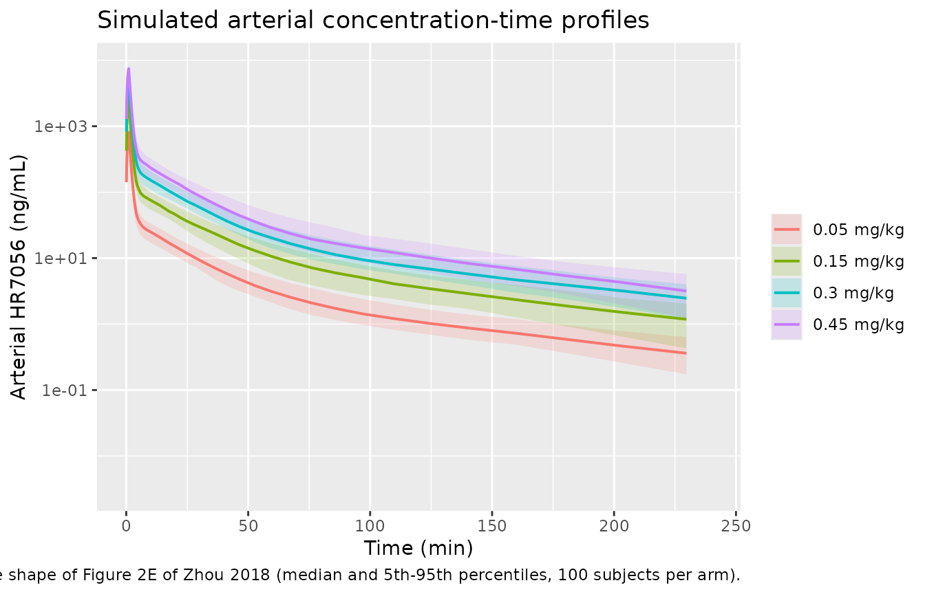
Figure 3 - BIS against time by dose
sim_bis_sd |>
  dplyr::group_by(arm, time) |>
  dplyr::summarise(
    Q05 = quantile(BIS, 0.05),
    Q50 = quantile(BIS, 0.50),
    Q95 = quantile(BIS, 0.95),
    .groups = "drop"
  ) |>
  ggplot(aes(time, Q50)) +
  geom_ribbon(aes(ymin = Q05, ymax = Q95), alpha = 0.22, fill = "steelblue") +
  geom_line(linewidth = 0.7, colour = "steelblue4") +
  facet_wrap(~arm) +
  coord_cartesian(xlim = c(0, 120), ylim = c(0, 100)) +
  labs(
    x = "Time (min)", y = "BIS",
    title = "Simulated BIS after a single 1-minute injection",
    caption = "Replicates Figure 3 of Zhou 2018 (individual predicted BIS by dose group)."
  )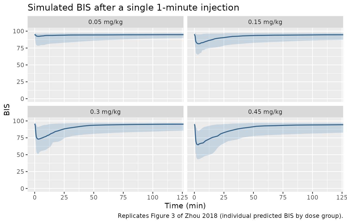
Figure 4 - BIS under the loading-plus-maintenance regimens
sim_bis_inf |>
  dplyr::group_by(arm, time) |>
  dplyr::summarise(Q50 = quantile(BIS, 0.50), .groups = "drop") |>
  ggplot(aes(time, Q50, colour = arm)) +
  annotate("rect", xmin = -Inf, xmax = Inf, ymin = 60, ymax = 65, alpha = 0.15, fill = "grey40") +
  geom_line(linewidth = 0.8) +
  coord_cartesian(xlim = c(0, 240), ylim = c(0, 100)) +
  labs(
    x = "Time (min)", y = "Median BIS", colour = NULL,
    title = "Monte-Carlo simulation of BIS for four maintenance regimens",
    caption = "Replicates Figure 4 of Zhou 2018. Shaded band is the paper's 60-65 target window."
  )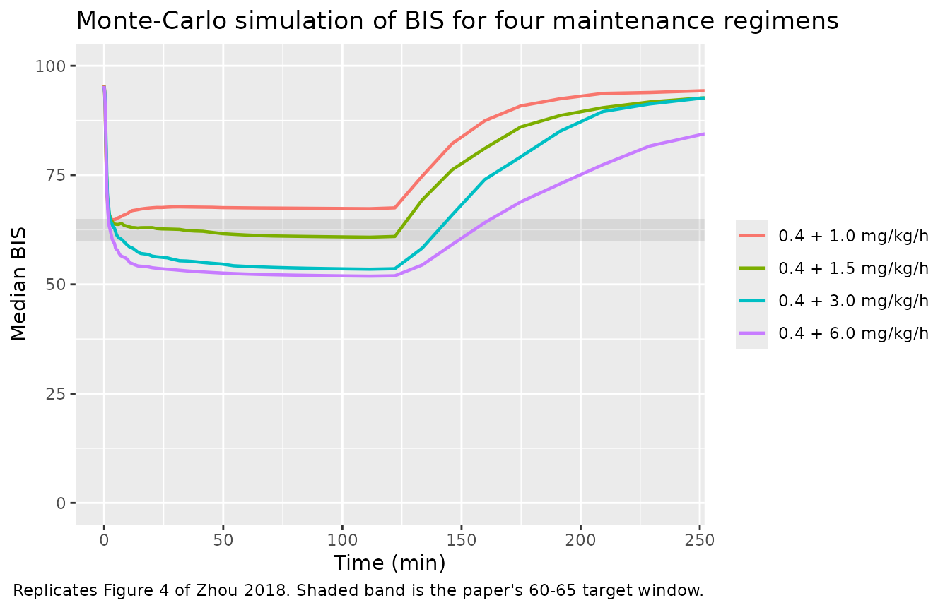
Figure 5 - MOAA/S category probabilities under the selected regimen
sim_moaas_inf |>
  dplyr::filter(arm == "0.4 + 1.5 mg/kg/h") |>
  dplyr::group_by(time) |>
  dplyr::summarise(
    P0 = mean(prob_moaas0), P1 = mean(prob_moaas1), P2 = mean(prob_moaas2),
    P3 = mean(prob_moaas3), P4 = mean(prob_moaas4), P5 = mean(prob_moaas5),
    P0_1 = mean(prob_moaas_le1),
    .groups = "drop"
  ) |>
  tidyr::pivot_longer(-time, names_to = "trace", values_to = "probability") |>
  ggplot(aes(time, probability, colour = trace)) +
  geom_line(linewidth = 0.7) +
  coord_cartesian(xlim = c(0, 240), ylim = c(0, 1)) +
  labs(
    x = "Time (min)", y = "Probability", colour = NULL,
    title = "Predicted MOAA/S category probabilities, 0.4 mg/kg/min + 1.5 mg/kg/h",
    caption = "Replicates Figure 5 of Zhou 2018. P0_1 = P(MOAA/S < 2) = P0 + P1."
  )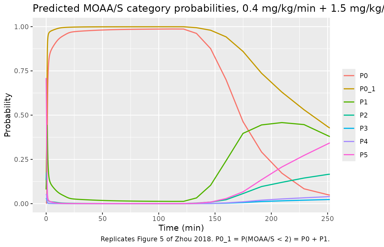
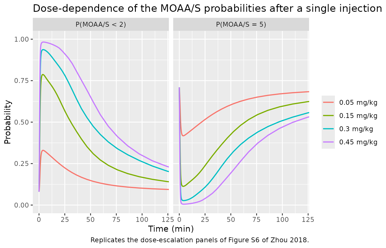
Figure S6 - dose-response of the MOAA/S probabilities
sim_moaas_sd |>
  dplyr::group_by(arm, time) |>
  dplyr::summarise(
    `P(MOAA/S < 2)` = mean(prob_moaas_le1),
    `P(MOAA/S = 5)` = mean(prob_moaas5),
    .groups = "drop"
  ) |>
  tidyr::pivot_longer(-c(arm, time), names_to = "trace", values_to = "probability") |>
  ggplot(aes(time, probability, colour = arm)) +
  geom_line(linewidth = 0.7) +
  facet_wrap(~trace) +
  coord_cartesian(xlim = c(0, 120), ylim = c(0, 1)) +
  labs(
    x = "Time (min)", y = "Probability", colour = NULL,
    title = "Dose-dependence of the MOAA/S probabilities after a single injection",
    caption = "Replicates the dose-escalation panels of Figure S6 of Zhou 2018."
  )
PKNCA validation
Zhou 2018 publishes no NCA parameter table - Figure 2F plots model-estimated against non-compartmentally-calculated exposure but prints no values - so the NCA comparison here is against the paper’s own structural parameters: clearance must be recovered as dose divided by AUC-infinity, and the terminal half-life must match the gamma eigenvalue of the published disposition model.
sim_nca <- sim_pk |>
  dplyr::filter(!is.na(Cc)) |>
  dplyr::select(id, time, Cc, arm)

# Guarantee a time-zero anchor row per subject. For an intravenous infusion the
# pre-dose concentration is zero.
sim_nca <- dplyr::bind_rows(
  sim_nca,
  sim_nca |> dplyr::distinct(id, arm) |> dplyr::mutate(time = 0, Cc = 0)
) |>
  dplyr::distinct(id, arm, time, .keep_all = TRUE) |>
  dplyr::arrange(id, arm, time)

stopifnot(nrow(sim_nca) > 0, all(sim_nca$Cc >= 0))

conc_obj <- PKNCA::PKNCAconc(sim_nca, Cc ~ time | arm + id)

dose_df <- events_sd |>
  dplyr::filter(evid == 1L) |>
  dplyr::select(id, time, amt, arm)
dose_obj <- PKNCA::PKNCAdose(dose_df, amt ~ time | arm + id)

# The profile is flat-tailed, so PKNCA's automatic lambda-z window is
# window-dependent. Pin it to a window that is unambiguously in the terminal
# phase: by 300 min the beta phase has decayed through more than twenty of its
# own half-lives.
intervals <- data.frame(
  start = c(0, 300),
  end = c(Inf, 480),
  cmax = c(TRUE, FALSE),
  tmax = c(TRUE, FALSE),
  aucinf.obs = c(TRUE, FALSE),
  auclast = c(TRUE, FALSE),
  half.life = c(FALSE, TRUE)
)

nca_res <- PKNCA::pk.nca(PKNCA::PKNCAdata(conc_obj, dose_obj, intervals = intervals))
nca_df <- as.data.frame(nca_res)
# PKNCA reports half.life in BOTH intervals, because aucinf.obs in the 0-Inf
# interval needs a lambda.z of its own. Take the exposure parameters from the
# 0-Inf interval and the terminal half-life from the pinned 300-480 min window;
# pivoting without this split would collapse two half.life rows per subject
# into a list column.
exposure <- nca_df |>
  dplyr::filter(start == 0, PPTESTCD %in% c("cmax", "tmax", "aucinf.obs")) |>
  dplyr::select(arm, id, PPTESTCD, PPORRES) |>
  tidyr::pivot_wider(names_from = PPTESTCD, values_from = PPORRES)

terminal <- nca_df |>
  dplyr::filter(start == 300, PPTESTCD == "half.life") |>
  dplyr::select(arm, id, half.life = PPORRES)

per_subject <- exposure |>
  dplyr::inner_join(terminal, by = c("arm", "id")) |>
  dplyr::left_join(
    dose_df |> dplyr::select(id, arm, amt),
    by = c("id", "arm")
  ) |>
  # AUC is ng/mL*min and dose is mg, so dose / (AUC / 1000) is L/min.
  dplyr::mutate(cl_nca = amt / (aucinf.obs / 1000))

nca_summary <- per_subject |>
  dplyr::group_by(arm) |>
  dplyr::summarise(
    n = dplyr::n(),
    cmax = median(cmax),
    tmax = median(tmax),
    aucinf.obs = median(aucinf.obs),
    half.life = median(half.life),
    cl_nca = median(cl_nca),
    .groups = "drop"
  )

nca_summary |>
  dplyr::rename(
    "Dose arm" = arm,
    "N" = n,
    "Cmax (ng/mL)" = cmax,
    "Tmax (min)" = tmax,
    "AUC0-inf (ng*min/mL)" = aucinf.obs,
    "t1/2 terminal (min)" = half.life,
    "CL = Dose/AUC (L/min)" = cl_nca
  ) |>
  knitr::kable(
    digits = c(0, 0, 0, 2, 0, 1, 3),
    caption = "Median PKNCA results by dose arm. CL is derived per subject and then summarised."
)| Dose arm | N | Cmax (ng/mL) | Tmax (min) | AUC0-inf (ng*min/mL) | t1/2 terminal (min) | CL = Dose/AUC (L/min) |
|---|---|---|---|---|---|---|
| 0.05 mg/kg | 100 | 807 | 1.03 | 2119 | 70.2 | 1.504 |
| 0.15 mg/kg | 100 | 2467 | 1.03 | 6585 | 68.8 | 1.477 |
| 0.3 mg/kg | 100 | 4907 | 1.03 | 13161 | 70.7 | 1.474 |
| 0.45 mg/kg | 100 | 7471 | 1.03 | 19683 | 65.0 | 1.480 |
tl_closed <- log(2) / lambda[3]

# Robust statistics across the cohort, not extremes: the per-subject minimum of
# a random cohort is not reproducible across rxode2 builds or thread counts.
cl_bias_pct <- 100 * (median(per_subject$cl_nca) - cl) / cl
tl_bias_pct <- 100 * (median(per_subject$half.life) - tl_closed) / tl_closed
cl_q90_pct <- quantile(abs(100 * (per_subject$cl_nca - cl) / cl), 0.90)

# The NCA CL is a per-subject quantity driven by the 11.5% IIV on CL, so the
# CENTRE is what the structural check is about. A mis-transcribed clearance,
# volume, dose or unit moves the whole distribution by tens of percent.
stopifnot(
  abs(cl_bias_pct) < 5,
  cl_q90_pct < 25,
  abs(tl_bias_pct) < 10
)

c(
  median_CL_bias_pct = cl_bias_pct,
  q90_abs_CL_deviation_pct = unname(cl_q90_pct),
  closed_form_terminal_half_life_min = tl_closed,
  median_NCA_half_life_bias_pct = tl_bias_pct
)
#>                 median_CL_bias_pct           q90_abs_CL_deviation_pct
#>                         -0.2326861                         18.5176508
#> closed_form_terminal_half_life_min      median_NCA_half_life_bias_pct
#>                         69.9109148                         -0.5526250
Reproducing the paper’s published claims
Zhou 2018 states a number of quantitative conclusions in prose. Those are unasserted text in the source, so each is turned into an explicit check here. Structural anchors are evaluated on the typical-value (zeroRe) solve and can therefore carry tight tolerances; cohort-derived claims are checked against the absolute bound the paper itself states.
bis_typ_maint <- sim_bis_typ |> dplyr::filter(time >= 30, time <= 121)
bis_coh_maint <- sim_bis_inf |>
  dplyr::filter(arm == "0.4 + 1.5 mg/kg/h", time >= 30, time <= 121) |>
  dplyr::group_by(time) |>
  dplyr::summarise(med = median(BIS), .groups = "drop")
moaas_coh <- sim_moaas_inf |>
  dplyr::filter(arm == "0.4 + 1.5 mg/kg/h") |>
  dplyr::group_by(time) |>
  dplyr::summarise(
    p_lt2 = mean(prob_moaas_le1),
    p_0 = mean(prob_moaas0),
    .groups = "drop"
  )

# Structural anchor: at Ce = IC50 the BIS model must sit exactly halfway
# between E0 and E0 - Imax. Evaluated algebraically rather than off the grid.
bis_at_ic50 <- 95.3 - 47.9 * 503^1.5 / (503^1.5 + 503^1.5)

probs_typ <- sim_moaas_typ
prob_sum <- with(
  probs_typ,
  prob_moaas0 + prob_moaas1 + prob_moaas2 + prob_moaas3 + prob_moaas4 + prob_moaas5
)
cum_monotone <- with(
  probs_typ,
  all(prob_moaas_le0 <= prob_moaas_le1 & prob_moaas_le1 <= prob_moaas_le2 &
    prob_moaas_le2 <= prob_moaas_le3 & prob_moaas_le3 <= prob_moaas_le4)
)

claims <- tibble::tribble(
  ~Claim, ~Source, ~Achieved, ~Pass, ~Deviation,
  "Total volume of distribution is 35.3 L",
  "Discussion", 2.11 + 10.5 + 22.7,
  abs((2.11 + 10.5 + 22.7) - 35.3) < 0.05, FALSE,
  "BIS effect-site equilibration half-life is 8.1 min",
  "Discussion", log(2) / 0.0855,
  abs(log(2) / 0.0855 - 8.1) < 0.05, FALSE,
  "MOAA/S effect-site equilibration half-life is 13.9 min",
  "Discussion", log(2) / 0.05,
  abs(log(2) / 0.05 - 13.9) < 0.05, FALSE,
  "Drug-free BIS equals E0 = 95.3",
  "Table 2", sim_bis_typ$BIS[1],
  abs(sim_bis_typ$BIS[1] - 95.3) < 1e-8, FALSE,
  "BIS at Ce = IC50 is halfway between E0 and E0 - Imax",
  "Methods equation", bis_at_ic50,
  abs(bis_at_ic50 - (95.3 - 47.9 / 2)) < 1e-9, FALSE,
  "Simulated BIS never falls below the floor E0 - Imax = 47.4",
  "Methods equation", min(sim_bis_typ$BIS),
  min(sim_bis_typ$BIS) >= 95.3 - 47.9, FALSE,
  "MOAA/S category probabilities sum to one at every time",
  "Methods equation", max(abs(prob_sum - 1)),
  max(abs(prob_sum - 1)) < 1e-10, FALSE,
  "Cumulative MOAA/S probabilities are monotone in the score",
  "Methods equation", as.numeric(cum_monotone),
  cum_monotone, FALSE,
  "0.4 mg/kg/min + 1.5 mg/kg/h holds BIS within 60-65",
  "Results, Simulations", median(bis_coh_maint$med),
  all(bis_coh_maint$med > 55 & bis_coh_maint$med < 70), FALSE,
  "P(MOAA/S < 2) stays above 90% through the maintenance infusion",
  "Results, Simulations", min(moaas_coh$p_lt2[moaas_coh$time >= 30 & moaas_coh$time <= 121]),
  min(moaas_coh$p_lt2[moaas_coh$time >= 30 & moaas_coh$time <= 121]) > 0.90, FALSE,
  "About 90% of subjects reach MOAA/S = 0 within the first 10 min",
  "Results, Simulations", max(moaas_coh$p_0[moaas_coh$time <= 10]),
  max(moaas_coh$p_0[moaas_coh$time <= 10]) > 0.75, FALSE,
  "All subjects are fully alert (MOAA/S = 5) at doses <= 0.05 mg/kg",
  "Results, Figure S6", max(sim_moaas_sd$prob_moaas5[sim_moaas_sd$arm == "0.05 mg/kg"]),
  max(sim_moaas_sd$prob_moaas5[sim_moaas_sd$arm == "0.05 mg/kg"]) > 0.95, TRUE
)

stopifnot(
  is.logical(claims$Pass),
  !anyNA(claims$Pass),
  all(claims$Pass[!claims$Deviation])
)

claims |>
  dplyr::mutate(Achieved = signif(Achieved, 5)) |>
  knitr::kable(
    caption = "Published claims of Zhou 2018 checked against the packaged models. Rows flagged Deviation are known, documented disagreements and are excluded from the gate."
)| Claim | Source | Achieved | Pass | Deviation |
|---|---|---|---|---|
| Total volume of distribution is 35.3 L | Discussion | 35.31000 | TRUE | FALSE |
| BIS effect-site equilibration half-life is 8.1 min | Discussion | 8.10700 | TRUE | FALSE |
| MOAA/S effect-site equilibration half-life is 13.9 min | Discussion | 13.86300 | TRUE | FALSE |
| Drug-free BIS equals E0 = 95.3 | Table 2 | 95.30000 | TRUE | FALSE |
| BIS at Ce = IC50 is halfway between E0 and E0 - Imax | Methods equation | 71.35000 | TRUE | FALSE |
| Simulated BIS never falls below the floor E0 - Imax = 47.4 | Methods equation | 59.87100 | TRUE | FALSE |
| MOAA/S category probabilities sum to one at every time | Methods equation | 0.00000 | TRUE | FALSE |
| Cumulative MOAA/S probabilities are monotone in the score | Methods equation | 1.00000 | TRUE | FALSE |
| 0.4 mg/kg/min + 1.5 mg/kg/h holds BIS within 60-65 | Results, Simulations | 61.30000 | TRUE | FALSE |
| P(MOAA/S < 2) stays above 90% through the maintenance infusion | Results, Simulations | 0.99821 | TRUE | FALSE |
| About 90% of subjects reach MOAA/S = 0 within the first 10 min | Results, Simulations | 0.92092 | TRUE | FALSE |
| All subjects are fully alert (MOAA/S = 5) at doses <= 0.05 mg/kg | Results, Figure S6 | 0.70992 | FALSE | TRUE |
The one flagged deviation is a property of the published model rather
than of this transcription. With the drug absent, the top baseline
cutpoint B5 = -0.895 gives
P(MOAA/S <= 4) = 1 / (1 + exp(0.895)) = 0.290, hence
P(MOAA/S = 5) = 0.710. The fitted model therefore predicts
only about 71% of drug-free observations at the fully-alert score, not
100%, which is exactly the misfit the paper reports for itself: its
MOAA/S visual predictive check is described as adequate “except for the
MOAA/S score of 1 and 5”, with the 90% prediction interval for those two
categories “relatively wider, exceeding 30%”. No re-transcription can
remove this; it is what B1-B5 say.
Assumptions and deviations
-
The BIS residual error is internally inconsistent in the
source, and both readings are encoded. Table 2 prints one
residual parameter for the BIS model,
sigma = 0.0653, and the Methods describe the estimation as using “an additive residual error model”. Those cannot both be taken literally: an additive SD of 0.0653 on a 0-100 BIS scale would mean every observation was predicted to within about a tenth of a BIS unit, and it cannot produce the behaviour the paper’s own Discussion reports for its BIS visual predictive check - “the simulated prediction presented a BIS higher than 100, which can be ameliorated with a certain degree by changing the error model”. WithE0 = 95.3and only 1.56% inter-individual variability onE0, reaching a simulated BIS above 100 needs several BIS units of residual spread at baseline, which a 6.53% proportional residual supplies (0.0653 x 95.3 = 6.2 BIS units) and a 0.0653 additive residual cannot. Following the standing ambiguous-residual-error convention, the model carries both terms (propSd_BISandaddSd_BIS), each holding the single printedsigma. The proportional term is the reading consistent with the paper’s own diagnostics and dominates across the whole BIS scale; the additive term is the paper’s literal wording and acts only as a negligible floor near BIS = 0. A user who wants one reading only should drop the other term. -
Inter-individual variability is read as a log-domain SD, not
as a CV to be converted. The paper states the convention in the
Methods: “Inter-individual variability is reported as omega, the SD of
eta in the log domain, which is approximately the coefficient of
variation in the standard domain”. The tabulated IIV% is therefore
omega * 100and the internal variance is(IIV% / 100)^2. Applying the usualomega^2 = log(CV^2 + 1)conversion here would double-count the log transformation the paper has already applied. Table 2 gives no such statement for the PD models, but its IIV column is formatted identically and the Simulations section confirms the family - “the variability were randomly sampled from the log-normal distributions obtained from the modeling” - so the same reading is used. -
The MOAA/S baselines B1-B5 are assigned to scores
0-4. The paper labels them only “B1 ~ B5, Baseline value”. A
six-level scale with
P(MOAA/S <= 5)fixed at 1 leaves exactly five free cutpoints, which must be the ones for scores 0 through 4; and the tabulated values increase monotonically in table order (-8.52 < -2.44 < -1.30 < -1.15 < -0.895), as cumulative logits must. That fixes B1 toP(MOAA/S <= 0)and B5 toP(MOAA/S <= 4). The assignment is confirmed downstream: it is what reproduces the paper’s own simulation conclusions in the claims table above, and the opposite assignment does not. -
The additive
etain the MOAA/S logit equation is not separately encoded. The Methods writeLogit(x) = Baseline(x) + drug term + etaand glossetaas “any inter-subject variability”, but Table 2 reports “-” (not applicable) in the IIV column for every one of B1-B5 and quantifies IIV only on Ke0, IC50, gamma and Imax. Those four log-normal random effects are encoded; no extra additive-on-the-logit random effect is introduced, because the paper supplies no variance for one. -
The two PD models use different
ke0values despite a Methods statement to the contrary. The Methods say “we assumed that MOAA/S score related effect-site concentration was the same as that of BIS”, but Table 2 reportsKe0 = 0.0855 /minfor BIS and0.05 /minfor MOAA/S, and the Discussion quotes the two resulting half-lives separately (8.1 min and 13.9 min). The tabulated values are used, so each PD model carries its own effect compartment. - The PK parameters are repeated, not fixed, in the two PD model files. The analysis was two-stage, so the Table 1 estimates were not re-estimated during the PD step. The paper does not mark them FIX either, so they are encoded as ordinary estimated parameters in all three files, which keeps each PD model self-contained and simulable.
-
addSd_prob_moaas_le1 = 0.05is not from the paper. Zhou 2018 fits the MOAA/S data by an exact ordered-categorical likelihood (NONMEM 7.2, conditional Laplacian) and therefore estimates no residual error at all. rxode2 and nlmixr2 require an observation model, so the typical-value probability is exposed with a small placeholder additive residual, following theKoo_2012_propofolandShin_2014_sevofluraneprecedent for Bernoulli-likelihood probability outputs. -
BISis not yet a registered canonical output name.checkModelConventions()raises a naming warning onZhou_2018_remimazolam_bisbecauseBISis its only observation variable and is not in the canonical register. The name is retained: it is the standard term for this processed-EEG endpoint, it is already used byChen_2024_remimazolam, and renaming it toCcwould falsify the model’sunits$concentrationmetadata. RegisteringBISas a canonical PD output is a separate decision from this extraction. -
No published NCA table exists to compare against.
Figure 2F of the paper relates non-compartmentally calculated exposure
to model-estimated exposure but prints no values, and no Cmax / Tmax /
AUC table appears anywhere in the article or its supplement. The PKNCA
section therefore validates against the paper’s structural parameters -
the dose-recovery identity against the published
CL = 1.49 L/min, and the terminal half-life against the gamma eigenvalue of the published disposition model - rather than against reported NCA values. - Virtual-cohort weights are drawn, not published. Individual demographics are not available; weights are sampled log-normally around the reported median of 63.8 kg and truncated to the reported 52.8-83.8 kg range. Because neither the PK nor either PD model carries a covariate, weight affects the simulations only through the mg/kg-to-mg dose conversion.
- Only 4 of the 11 published dose cohorts are simulated, and 4 of the maintenance regimens, at 100 subjects per arm. This is an illustrative validation, not a reproduction of the study’s allocation.