Ritlecitinib eyebrow and eyelash assessment exposure-response in alopecia areata (Wang 2025)
Source:vignettes/articles/Wang_2025_ritlecitinib_eyebrow_eyelash.Rmd
Wang_2025_ritlecitinib_eyebrow_eyelash.RmdModel and source
- Citation: Wang Y, Huh Y, Lejeune A. (2025). Population exposure-response analysis of the effect of ritlecitinib on eyebrow assessment and eyelash assessment in patients with alopecia areata. CPT: Pharmacometrics & Systems Pharmacology 14(2):389-402.
- Article: https://doi.org/10.1002/psp4.13283 (PMC11812936, open access). The supporting information includes both NONMEM control streams (Data S1 for the eyebrow model, Data S2 for the eyelash model), which this extraction follows for every equation.
The paper reports two independently fitted longitudinal exposure-response (ER) models, one for the eyebrow assessment (EBA) score and one for the eyelash assessment (ELA) score, in participants of the phase 2b/3 study B7981015 whose eyebrows or eyelashes were abnormal at baseline. They are packaged as two models:
-
Wang_2025_ritlecitinib_eyebrow– EBA score; -
Wang_2025_ritlecitinib_eyelash– ELA score.
EBA and ELA are four-level ordinal scores: 0 = none, 1 = minimal, 2 =
moderate, 3 = normal eyebrows or eyelashes. Each model is a
cumulative-probit ordinal regression (Wang 2025 Eq
1-5). With PBO(t) the placebo effect and D(t)
the drug effect,
with B2 = exp(theta_2) and
B3 = exp(theta_3) so that the cut-offs stay ordered. The
drug effect is the latent variable of a stimulated-kin indirect response
(Eq 6-8), with kin = kout:
and the placebo effect is PBO(t) = Pmax (1 - exp(-k t))
(Eq 9-11), sharing the drug-effect rate k (Section 3.2).
The typical Pmax is fixed to zero, so the placebo effect is
purely between-subject variability.
There is no PK component: ritlecitinib exposure
enters as the CAV column, the average concentration between
adjacent EBA/ELA records, which the authors derived from the empirical
Bayes estimates of the ritlecitinib population PK model of Wojciechowski
2023 (packaged here as
Wojciechowski_2023_ritlecitinib_final). This vignette
chains the two: the PK model supplies CAV, and the ER
models turn it into score probabilities. The SALT-score model built on
the same exposure metric is Huh_2024_ritlecitinib.
eba <- readModelDb("Wang_2025_ritlecitinib_eyebrow")
ela <- readModelDb("Wang_2025_ritlecitinib_eyelash")
pk <- readModelDb("Wojciechowski_2023_ritlecitinib_final")
Population
Both analyses use study B7981015 (Wang 2025 Tables 1 and 2). Participants with a normal score at baseline were excluded, so the two analysis sets overlap but differ.
| Characteristic | EBA analysis (Table 1) | ELA analysis (Table 2) |
|---|---|---|
| Participants / observations | 594 / 5456 | 535 / 4929 |
| Age, median (range) | 33 (12, 72) years | 33 (12, 72) years |
| Weight, median (range) | 68.3 (35.0, 200.0) kg | 68.7 (35.0, 200.0) kg |
| Female | 355 (59.8%) | 313 (58.5%) |
| Race | White 67.0%, Asian 26.9%, Black 3.5%, Other 2.5% | White 67.9%, Asian 26.5%, Black 3.2%, Other 2.4% |
| Region | North America 40.2%, Europe 21.9%, Asia 21.5%, Rest of World 16.3% | North America 41.3%, Europe 22.6%, Asia 20.6%, Rest of World 15.5% |
| Baseline score 0 / 1 / 2 | 55.2% / 30.6% / 14.1% | 52.9% / 31.0% / 16.1% |
The arms were 200 mg QD for 4 weeks then 50 or 30 mg QD, 50, 30 or 10
mg QD for 48 weeks, and placebo for 24 weeks followed by 200/50 or 50 mg
QD. The same metadata is available programmatically via
readModelDb(...)$population.
Source trace
| Model element | EBA value | ELA value | Source location |
|---|---|---|---|
| Cumulative-probit ordinal structure | – | – | Eq 1-5; control streams $ERROR
|
Cut-offs alpha_2 = B1, alpha_1 = B1 - B2,
alpha_0 = B1 - B2 - B3
|
– | – | Eq 2; control streams A2, A1,
A0
|
B2 = exp(THETA(2)),
B3 = exp(THETA(3))
|
– | – | Control streams $PK
|
| Drug effect subtracted, placebo effect added | – | – | Control streams $ERROR (see Errata) |
Stimulated-kin indirect response, A(0) = 1
|
– | – | Eq 6-8; control streams $DES,
A_0(1) = 1
|
kin = kout; placebo rate = drug rate |
– | – | Section 3.2; control streams POPDEKON,
POPPBOKON
|
Placebo effect Pmax (1 - exp(-k t))
|
– | – | Eq 9-11; control streams PBOEFF
|
b1 |
6.05 | 7.31 | Tables 3 and 4, “Baseline (B1)” |
lb2 |
1.01 | 1.12 | Tables 3 and 4, “Difference in baselines for score 3 and score 2 (B2)” |
lb3 |
1.11 | 1.18 | Tables 3 and 4, “Difference in baselines for score 2 and score 1 (B3)” |
pmax |
0 (fixed) | 0 (fixed) | Section 3.2; control streams POPPMAX = 0
|
emax |
11.0 | 7.75 | Tables 3 and 4, “Maximum Drug effect (Emax)” |
ec50 |
exp(10.6)/1000 = 40.1 ng/mL | exp(10.2)/1000 = 26.9 ng/mL | Tables 3 and 4, EC50 row and footnote |
thalfrec_drug |
34.1 weeks | 27.3 weeks | Tables 3 and 4, “Half-Life of Drug Onset” and footnote |
e_race_asian_emax |
0.487 | 0.647 | Tables 3 and 4, “Effect of Asian on Emax”;
COVASIAN = 1 + THETA(7)
|
e_sexf_b1 |
– | -1.19 | Table 4, “Effect of Female on B1”;
IF(SEX.EQ.2) SEXB1 = THETA(8)
|
var(etab1) (additive) |
6.53 | 9.05 | Tables 3 and 4, omega^2 B1; Section 2.3.2 |
var(etalemax) (exponential) |
0.409 | 0.408 | Tables 3 and 4, omega^2 Emax; Section 2.3.2 |
var(etapmax) (additive) |
21.8 | 12.9 | Tables 3 and 4, omega^2 Pmax; Section 2.3.2 |
CAV definition |
– | – | Section 2.2 |
| Cavg of 50 mg QD = 52 ng/mL, of 30 mg QD = 27 ng/mL | – | – | Section 3.2 |
| Responder definition (>= 2-grade improvement or score 3) | – | – | Section 2.4 |
Exposure layer: Cavg from the packaged ritlecitinib population PK model
The paper anchors two steady-state Cavg values: 52 ng/mL for 50 mg QD and 27 ng/mL for 30 mg QD (Section 3.2). We reproduce both and generate Cavg for the other simulated doses by solving the packaged Wojciechowski 2023 final PK model at its typical values for a 70 kg alopecia areata patient, then taking the steady-state average concentration over a dosing interval with PKNCA. The PK model has an autoinhibitory Imax term, so Cavg is not proportional to dose and cannot be scaled from 52 ng/mL.
doseLevels <- c(10, 30, 50, 100, 200, 300, 400, 500, 600)
tau <- 24        # h, once daily
nDays <- 21      # dosing days before the evaluated interval

# zeroRe() warns that the PK model's etas are not mu-referenced, which does
# not affect a typical-value solve.
pkTypical <- suppressWarnings(rxode2::zeroRe(pk))
#> ℹ parameter labels from comments will be replaced by 'label()'

pkEvents <- lapply(seq_along(doseLevels), function(k) {
  ev <- rxode2::et(amt = doseLevels[k], ii = tau, until = tau * nDays,
                   cmt = "depot") %>%
    rxode2::et(seq(tau * nDays, tau * (nDays + 1), by = 0.25))
  as.data.frame(ev) %>%
    dplyr::mutate(id = k)
}) %>%
  dplyr::bind_rows() %>%
  dplyr::mutate(WT = 70, DIS_ALOPECIA_AREATA = 1, RENALIMP_SEV = 0)

# One typical subject per dose level, so the no-omega warning is expected.
pkSolve <- suppressWarnings(
  rxode2::rxSolve(pkTypical, pkEvents, returnType = "data.frame")
)
#> ℹ omega/sigma items treated as zero: 'etalcl', 'etalvc'

pkConc <- pkSolve %>%
  dplyr::filter(time >= tau * nDays, !is.na(Cc)) %>%
  dplyr::mutate(
    # `doseLevel`, not `dose`: PKNCA treats `dose` as a reserved column name in
    # the concentration frame.
    doseLevel = doseLevels[as.integer(id)],
    treatment = paste0(doseLevel, " mg QD"),
    time = time - tau * nDays,
    id = as.integer(id)
  )

pkDose <- pkConc %>%
  dplyr::group_by(treatment, id) %>%
  dplyr::summarise(dose = dplyr::first(doseLevel), .groups = "drop") %>%
  dplyr::mutate(time = 0)

concObj <- PKNCA::PKNCAconc(pkConc, Cc ~ time | treatment + id)
doseObj <- PKNCA::PKNCAdose(pkDose, dose ~ time | treatment + id)
ivals <- data.frame(start = 0, end = tau, cav = TRUE, cmax = TRUE, cmin = TRUE)
ncaRes <- PKNCA::pk.nca(PKNCA::PKNCAdata(concObj, doseObj, intervals = ivals))

cavgTable <- as.data.frame(ncaRes) %>%
  dplyr::filter(PPTESTCD == "cav") %>%
  dplyr::select(treatment, cav = PPORRES) %>%
  dplyr::mutate(dose = as.numeric(sub(" mg QD", "", treatment, fixed = TRUE))) %>%
  dplyr::arrange(dose)

cavgTable %>%
  dplyr::mutate(cav = round(cav, 1)) %>%
  dplyr::select(dose, cav) %>%
  dplyr::rename(`Dose (mg QD)` = dose, `Steady-state Cavg (ng/mL)` = cav) %>%
knitr::kable(caption = "Steady-state Cavg by ritlecitinib dose, typical values of the Wojciechowski 2023 final PK model (70 kg, alopecia areata).")| Dose (mg QD) | Steady-state Cavg (ng/mL) |
|---|---|
| 10 | 6.5 |
| 30 | 26.4 |
| 50 | 51.0 |
| 100 | 117.6 |
| 200 | 254.4 |
| 300 | 391.9 |
| 400 | 529.5 |
| 500 | 667.2 |
| 600 | 805.0 |
cavOf <- function(dose) cavgTable$cav[cavgTable$dose == dose]
cavCheck <- data.frame(
  dose = c(30, 50),
  published = c(27, 52),
  simulated = c(cavOf(30), cavOf(50))
) %>%
  dplyr::mutate(pct_diff = 100 * (simulated - published) / published)
knitr::kable(cavCheck, digits = 1)| dose | published | simulated | pct_diff |
|---|---|---|---|
| 30 | 27 | 26.4 | -2.4 |
| 50 | 52 | 51.0 | -1.9 |
# Structural: a mis-transcribed clearance, dose or unit in either packaged model
# moves these by tens of percent. The 10% band leaves room for the published
# values being cohort summaries over EBEs rather than a typical-value solve.
stopifnot(all(abs(cavCheck$pct_diff) < 10))
The EC50 estimates sit at these anchors, which is the paper’s explanation for why a 200 mg loading dose helps the eyebrow score more than the eyelash score: the eyebrow EC50 (40.1 ng/mL) lies near the 50 mg QD Cavg, while the eyelash EC50 (26.9 ng/mL) lies near the 30 mg QD Cavg (Section 4.2).
Structural identities
These checks use typical values, so both sides of every comparison use the same parameters and any difference is pure numerical error; they are asserted tightly.
solveTypical <- function(mod, cav, weeks, covs = list()) {
  ev <- data.frame(id = 1L, time = weeks, CAV = cav)
  for (nm in names(covs)) ev[[nm]] <- covs[[nm]]
  # The ordinal models have no sigma, so zeroRe() warns; harmless here.
  rxode2::rxSolve(suppressWarnings(rxode2::zeroRe(mod)), ev,
                  returnType = "data.frame")
}

typical <- list(
  EBA = list(mod = eba, b1 = 6.05, b2 = exp(1.01), b3 = exp(1.11), emax = 11.0,
             ec50 = exp(10.6) / 1000, thalf = 34.1,
             covs = list(RACE_ASIAN = 0)),
  ELA = list(mod = ela, b1 = 7.31, b2 = exp(1.12), b3 = exp(1.18), emax = 7.75,
             ec50 = exp(10.2) / 1000, thalf = 27.3,
             covs = list(RACE_ASIAN = 0, SEXF = 0))
)

for (nm in names(typical)) {
  p <- typical[[nm]]

  # 1. Untreated: the latent variable stays at 1 and, with the typical Pmax of
  # zero, the score probabilities are the closed-form cut-off probabilities.
  hold <- solveTypical(p$mod, cav = 0, weeks = c(0, 12, 48), covs = p$covs)
  stopifnot(
    max(abs(hold$effect - 1)) < 1e-10,
    max(abs(hold$p0 - pnorm(p$b1 - p$b2 - p$b3))) < 1e-10,
    max(abs(hold$p3 - (1 - pnorm(p$b1)))) < 1e-10
  )

  # 2. At CAV = EC50 the latent variable settles at 1 + Emax/2.
  half <- solveTypical(p$mod, cav = p$ec50, weeks = c(0, 2000), covs = p$covs)
  stopifnot(abs(dplyr::last(half$effect) - (1 + p$emax / 2)) < 1e-4)

  # 3. Under constant saturating exposure the latent variable reaches half of
  # its final rise at the published onset half-life (weeks).
  sat <- solveTypical(p$mod, cav = 1e9, weeks = c(0, p$thalf), covs = p$covs)
  stopifnot(abs(dplyr::last(sat$effect) - (1 + p$emax / 2)) < 1e-4)
}
#> ℹ parameter labels from comments will be replaced by 'label()'
#> ℹ omega/sigma items treated as zero: 'etab1', 'etalemax', 'etapmax'
#> ℹ parameter labels from comments will be replaced by 'label()'
#> ℹ omega/sigma items treated as zero: 'etab1', 'etalemax', 'etapmax'
#> ℹ parameter labels from comments will be replaced by 'label()'
#> ℹ omega/sigma items treated as zero: 'etab1', 'etalemax', 'etapmax'
#> ℹ parameter labels from comments will be replaced by 'label()'
#> ℹ omega/sigma items treated as zero: 'etab1', 'etapmax', 'etalemax'
#> ℹ parameter labels from comments will be replaced by 'label()'
#> ℹ omega/sigma items treated as zero: 'etab1', 'etapmax', 'etalemax'
#> ℹ parameter labels from comments will be replaced by 'label()'
#> ℹ omega/sigma items treated as zero: 'etab1', 'etapmax', 'etalemax'
cat("Untreated hold, EC50 half-maximum and onset half-life identities hold for both models.\n")
#> Untreated hold, EC50 half-maximum and onset half-life identities hold for both models.
Baseline score distribution (Tables 1, 2 and S3)
The cut-offs and the additive B1 variability fully determine the
predicted baseline score distribution, so this is the most direct check
that B2 and B3 are the exponentials of the
tabulated values (the control stream’s B2 = EXP(THETA(2))).
Integrating the additive eta_B1 out of a probit gives
P(Y <= j) = Phi(alpha_j / sqrt(1 + omega^2_B1)). The
analysis sets excluded baseline score 3, so the prediction is
conditioned on Y < 3.
baselineDist <- function(b1, omega2, b2, b3) {
  den <- sqrt(1 + omega2)
  pc <- pnorm(c(b1 - b2 - b3, b1 - b2, b1) / den)
  p <- c(pc[1], diff(pc))
  100 * p / pc[3]
}
ebaPred <- baselineDist(6.05, 6.53, exp(1.01), exp(1.11))
elaMale <- baselineDist(7.31, 9.05, exp(1.12), exp(1.18))
elaFemale <- baselineDist(7.31 - 1.19, 9.05, exp(1.12), exp(1.18))
# Read as linear-scale gaps instead, the cut-offs put almost everyone at 0.
ebaLinear <- baselineDist(6.05, 6.53, 1.01, 1.11)

baseTab <- data.frame(
  group = rep(c("EBA, all (Table 1)", "ELA, male (Table S3)",
                "ELA, female (Table S3)", "EBA, gaps read as linear"), each = 3),
  score = rep(0:2, 4),
  observed = c(55.2, 30.6, 14.1, 62.2, 26.1, 11.7, 46.3, 34.5, 19.2,
               55.2, 30.6, 14.1),
  predicted = c(ebaPred, elaMale, elaFemale, ebaLinear)
)
baseTab %>%
  dplyr::mutate(predicted = round(predicted, 1)) %>%
  dplyr::rename(Group = group, `Baseline score` = score,
                `Observed (%)` = observed, `Predicted (%)` = predicted) %>%
knitr::kable(caption = "Observed versus model-predicted baseline score distribution, conditional on a baseline score below 3.")| Group | Baseline score | Observed (%) | Predicted (%) |
|---|---|---|---|
| EBA, all (Table 1) | 0 | 55.2 | 54.7 |
| EBA, all (Table 1) | 1 | 30.6 | 35.1 |
| EBA, all (Table 1) | 2 | 14.1 | 10.2 |
| ELA, male (Table S3) | 0 | 62.2 | 62.9 |
| ELA, male (Table S3) | 1 | 26.1 | 29.0 |
| ELA, male (Table S3) | 2 | 11.7 | 8.1 |
| ELA, female (Table S3) | 0 | 46.3 | 48.8 |
| ELA, female (Table S3) | 1 | 34.5 | 36.7 |
| ELA, female (Table S3) | 2 | 19.2 | 14.5 |
| EBA, gaps read as linear | 0 | 55.2 | 93.7 |
| EBA, gaps read as linear | 1 | 30.6 | 4.4 |
| EBA, gaps read as linear | 2 | 14.1 | 2.0 |
modelRows <- baseTab$group != "EBA, gaps read as linear"
stopifnot(
  # Every packaged-model category within 6 points of the observed share. The
  # linear-gap reading misses score 0 by almost 40 points.
  all(abs(baseTab$observed - baseTab$predicted)[modelRows] < 6),
  abs(ebaLinear[1] - 55.2) > 30,
  # The female shift on B1 moves eyelash scores up (less severe at baseline).
  elaFemale[1] < elaMale[1]
)
Virtual cohort
The paper simulated 1000 trials of 200 participants with the B7981015
demographic distribution and averaged Cavg over 4-week windows (Section
2.4). Here a single cohort of 200 participants per model is drawn
once, in base R, and reused for every regimen. Common
random numbers make the dose-response and loading-dose contrasts depend
only on the regimen, and a base-R set.seed() draws the same
cohort on every machine (rxode2’s own RNG stream depends on the solver
thread count). The Asian and female proportions follow Tables 1 and
2.
set.seed(20250214)
nSub <- 200L

ebaCohort <- data.frame(
  id = seq_len(nSub),
  RACE_ASIAN = as.integer(stats::runif(nSub) < 0.269),
  etab1 = stats::rnorm(nSub, 0, sqrt(6.53)),
  etalemax = stats::rnorm(nSub, 0, sqrt(0.409)),
  etapmax = stats::rnorm(nSub, 0, sqrt(21.8))
)
elaCohort <- data.frame(
  id = seq_len(nSub),
  RACE_ASIAN = as.integer(stats::runif(nSub) < 0.265),
  SEXF = as.integer(stats::runif(nSub) < 0.585),
  etab1 = stats::rnorm(nSub, 0, sqrt(9.05)),
  etalemax = stats::rnorm(nSub, 0, sqrt(0.408)),
  etapmax = stats::rnorm(nSub, 0, sqrt(12.9))
)

# Build a weekly event frame for a regimen given as a step function of Cavg:
# `schedule$from` (week) and `schedule$cav` (ng/mL).
makeEvents <- function(schedule, cohort, weeks = 0:48) {
  tidyr::expand_grid(id = cohort$id, time = weeks) %>%
    dplyr::left_join(cohort, by = "id") %>%
    dplyr::mutate(CAV = schedule$cav[findInterval(time, schedule$from)])
}

# Expected responder rate among participants with a baseline score below 3.
# Given the random effects, the scores at baseline and at week `wk` are
# independent draws, so with b the baseline score
#   P(responder, Y0 < 3) = sum_b P(Y0 = b) * P(Y_wk >= min(b + 2, 3)).
# Averaging these probabilities over the cohort, rather than drawing scores,
# removes the score-sampling noise from the comparison.
responderRate <- function(sim, wk) {
  b <- sim %>%
    dplyr::filter(time == 0) %>%
    dplyr::select(id, b0 = p0, b1 = p1, b2 = p2)
  w <- sim %>%
    dplyr::filter(time == wk) %>%
    dplyr::select(id, w2 = p2, w3 = p3)
  m <- dplyr::inner_join(b, w, by = "id")
  stopifnot(nrow(m) == nrow(b), nrow(m) > 0)
  num <- m$b0 * (m$w2 + m$w3) + (m$b1 + m$b2) * m$w3
  100 * sum(num) / sum(m$b0 + m$b1 + m$b2)
}

simRegimen <- function(mod, cohort, schedule) {
  # zeroRe() warns that the ordinal models have no sigma, and rxSolve() that
  # a multi-subject solve has no omega: both intended for a typical-value
  # cohort that differs only in covariates.
  suppressWarnings(rxode2::rxSolve(rxode2::zeroRe(mod),
                                  makeEvents(schedule, cohort),
                                  returnType = "data.frame"))
}
Replicating Figure 2: dose-response at weeks 24 and 48
Figure 2 of Wang 2025 shows the median simulated responder rate (at least a two-grade improvement, or a normal score) for placebo and 10-600 mg QD without a loading dose. The published medians are read from the bar labels.
fig2 <- data.frame(
  endpoint = rep(c("EBA", "ELA"), each = 20),
  week = rep(rep(c(24, 48), each = 10), 2),
  dose = rep(c(0, doseLevels), 4),
  published = c(
    4, 8.5, 21.5, 30.5, 41.5, 48, 50, 51.5, 52, 52.5,
    9.5, 19, 38.5, 50, 61, 67.5, 69.5, 70.5, 71, 71.5,
    3, 8.5, 20.5, 27.5, 35, 39.5, 41.5, 42, 42.5, 42.5,
    6.5, 17, 35.5, 45, 53.5, 58, 60, 60.5, 61, 61
  )
)

doseSims <- list()
for (d in c(0, doseLevels)) {
  cav <- if (d == 0) 0 else cavOf(d)
  sched <- data.frame(from = 0, cav = cav)
  doseSims[[paste("EBA", d)]] <- simRegimen(eba, ebaCohort, sched)
  doseSims[[paste("ELA", d)]] <- simRegimen(ela, elaCohort, sched)
}
#> ℹ parameter labels from comments will be replaced by 'label()'
#> ℹ omega/sigma items treated as zero: 'etab1', 'etalemax', 'etapmax'
#> ℹ parameter labels from comments will be replaced by 'label()'
#> ℹ omega/sigma items treated as zero: 'etab1', 'etapmax', 'etalemax'
#> ℹ parameter labels from comments will be replaced by 'label()'
#> ℹ omega/sigma items treated as zero: 'etab1', 'etalemax', 'etapmax'
#> ℹ parameter labels from comments will be replaced by 'label()'
#> ℹ omega/sigma items treated as zero: 'etab1', 'etapmax', 'etalemax'
#> ℹ parameter labels from comments will be replaced by 'label()'
#> ℹ omega/sigma items treated as zero: 'etab1', 'etalemax', 'etapmax'
#> ℹ parameter labels from comments will be replaced by 'label()'
#> ℹ omega/sigma items treated as zero: 'etab1', 'etapmax', 'etalemax'
#> ℹ parameter labels from comments will be replaced by 'label()'
#> ℹ omega/sigma items treated as zero: 'etab1', 'etalemax', 'etapmax'
#> ℹ parameter labels from comments will be replaced by 'label()'
#> ℹ omega/sigma items treated as zero: 'etab1', 'etapmax', 'etalemax'
#> ℹ parameter labels from comments will be replaced by 'label()'
#> ℹ omega/sigma items treated as zero: 'etab1', 'etalemax', 'etapmax'
#> ℹ parameter labels from comments will be replaced by 'label()'
#> ℹ omega/sigma items treated as zero: 'etab1', 'etapmax', 'etalemax'
#> ℹ parameter labels from comments will be replaced by 'label()'
#> ℹ omega/sigma items treated as zero: 'etab1', 'etalemax', 'etapmax'
#> ℹ parameter labels from comments will be replaced by 'label()'
#> ℹ omega/sigma items treated as zero: 'etab1', 'etapmax', 'etalemax'
#> ℹ parameter labels from comments will be replaced by 'label()'
#> ℹ omega/sigma items treated as zero: 'etab1', 'etalemax', 'etapmax'
#> ℹ parameter labels from comments will be replaced by 'label()'
#> ℹ omega/sigma items treated as zero: 'etab1', 'etapmax', 'etalemax'
#> ℹ parameter labels from comments will be replaced by 'label()'
#> ℹ omega/sigma items treated as zero: 'etab1', 'etalemax', 'etapmax'
#> ℹ parameter labels from comments will be replaced by 'label()'
#> ℹ omega/sigma items treated as zero: 'etab1', 'etapmax', 'etalemax'
#> ℹ parameter labels from comments will be replaced by 'label()'
#> ℹ omega/sigma items treated as zero: 'etab1', 'etalemax', 'etapmax'
#> ℹ parameter labels from comments will be replaced by 'label()'
#> ℹ omega/sigma items treated as zero: 'etab1', 'etapmax', 'etalemax'
#> ℹ parameter labels from comments will be replaced by 'label()'
#> ℹ omega/sigma items treated as zero: 'etab1', 'etalemax', 'etapmax'
#> ℹ parameter labels from comments will be replaced by 'label()'
#> ℹ omega/sigma items treated as zero: 'etab1', 'etapmax', 'etalemax'

fig2$simulated <- mapply(function(ep, wk, d) {
  responderRate(doseSims[[paste(ep, d)]], wk)
}, fig2$endpoint, fig2$week, fig2$dose)
fig2$diff <- fig2$simulated - fig2$published

ggplot(fig2, aes(factor(dose), simulated)) +
  geom_col(fill = "grey70") +
  geom_point(aes(y = published), colour = "firebrick", size = 2) +
  facet_grid(endpoint ~ paste("Week", week)) +
  labs(x = "Dose (mg QD; 0 = placebo)", y = "Responder rate (%)",
       caption = "Bars: this cohort. Red points: Wang 2025 Figure 2 medians.") +
  theme_bw()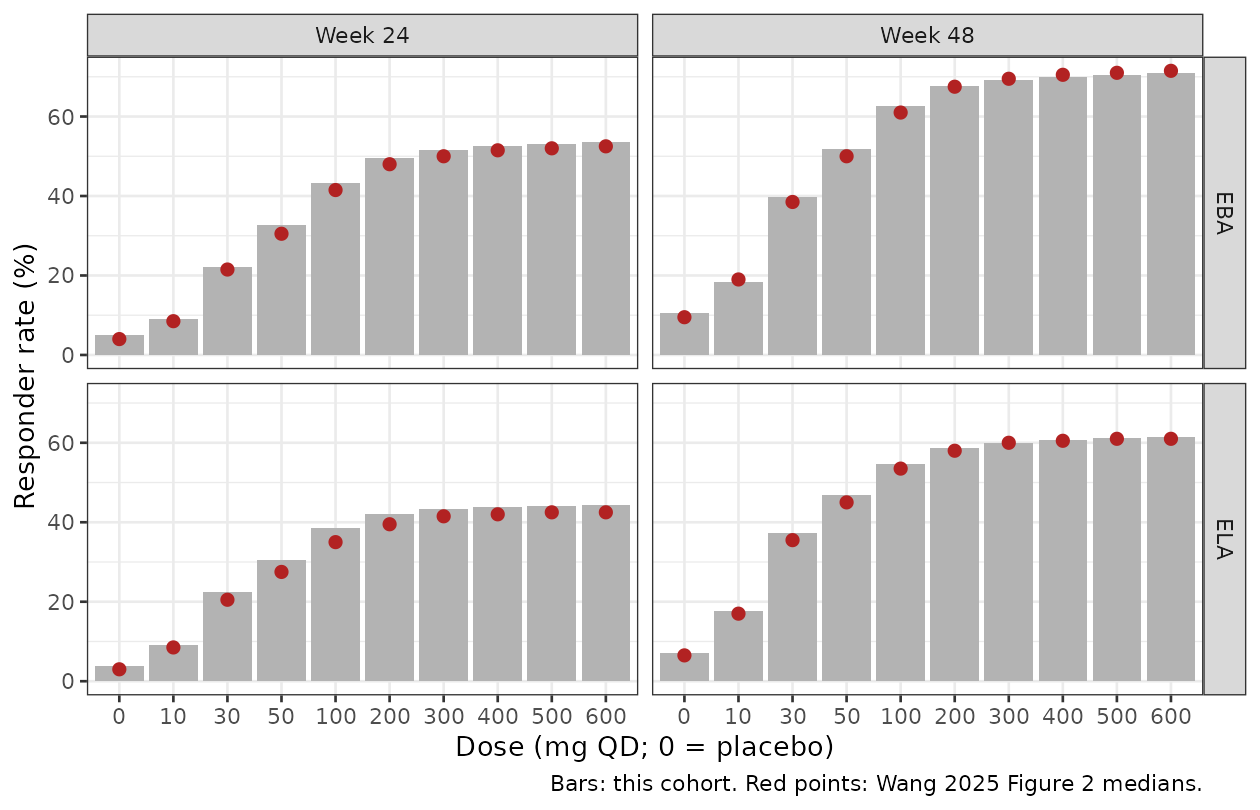
Replicates Figure 2 of Wang 2025.
fig2 %>%
  dplyr::mutate(simulated = round(simulated, 1), diff = round(diff, 1)) %>%
  dplyr::rename(Endpoint = endpoint, Week = week, `Dose (mg QD)` = dose,
                `Published (%)` = published, `Simulated (%)` = simulated,
                `Difference (points)` = diff) %>%
knitr::kable(caption = "Responder rates: Wang 2025 Figure 2 medians versus this cohort.")| Endpoint | Week | Dose (mg QD) | Published (%) | Simulated (%) | Difference (points) |
|---|---|---|---|---|---|
| EBA | 24 | 0 | 4.0 | 5.1 | 1.1 |
| EBA | 24 | 10 | 8.5 | 9.1 | 0.6 |
| EBA | 24 | 30 | 21.5 | 22.2 | 0.7 |
| EBA | 24 | 50 | 30.5 | 32.7 | 2.2 |
| EBA | 24 | 100 | 41.5 | 43.3 | 1.8 |
| EBA | 24 | 200 | 48.0 | 49.5 | 1.5 |
| EBA | 24 | 300 | 50.0 | 51.6 | 1.6 |
| EBA | 24 | 400 | 51.5 | 52.6 | 1.1 |
| EBA | 24 | 500 | 52.0 | 53.2 | 1.2 |
| EBA | 24 | 600 | 52.5 | 53.6 | 1.1 |
| EBA | 48 | 0 | 9.5 | 10.6 | 1.1 |
| EBA | 48 | 10 | 19.0 | 18.3 | -0.7 |
| EBA | 48 | 30 | 38.5 | 39.9 | 1.4 |
| EBA | 48 | 50 | 50.0 | 51.8 | 1.8 |
| EBA | 48 | 100 | 61.0 | 62.6 | 1.6 |
| EBA | 48 | 200 | 67.5 | 67.6 | 0.1 |
| EBA | 48 | 300 | 69.5 | 69.2 | -0.3 |
| EBA | 48 | 400 | 70.5 | 70.0 | -0.5 |
| EBA | 48 | 500 | 71.0 | 70.5 | -0.5 |
| EBA | 48 | 600 | 71.5 | 70.8 | -0.7 |
| ELA | 24 | 0 | 3.0 | 3.8 | 0.8 |
| ELA | 24 | 10 | 8.5 | 9.2 | 0.7 |
| ELA | 24 | 30 | 20.5 | 22.4 | 1.9 |
| ELA | 24 | 50 | 27.5 | 30.5 | 3.0 |
| ELA | 24 | 100 | 35.0 | 38.5 | 3.5 |
| ELA | 24 | 200 | 39.5 | 42.1 | 2.6 |
| ELA | 24 | 300 | 41.5 | 43.3 | 1.8 |
| ELA | 24 | 400 | 42.0 | 43.8 | 1.8 |
| ELA | 24 | 500 | 42.5 | 44.1 | 1.6 |
| ELA | 24 | 600 | 42.5 | 44.4 | 1.9 |
| ELA | 48 | 0 | 6.5 | 7.2 | 0.7 |
| ELA | 48 | 10 | 17.0 | 17.7 | 0.7 |
| ELA | 48 | 30 | 35.5 | 37.2 | 1.7 |
| ELA | 48 | 50 | 45.0 | 46.8 | 1.8 |
| ELA | 48 | 100 | 53.5 | 54.6 | 1.1 |
| ELA | 48 | 200 | 58.0 | 58.7 | 0.7 |
| ELA | 48 | 300 | 60.0 | 60.0 | 0.0 |
| ELA | 48 | 400 | 60.5 | 60.7 | 0.2 |
| ELA | 48 | 500 | 61.0 | 61.1 | 0.1 |
| ELA | 48 | 600 | 61.0 | 61.4 | 0.4 |
stopifnot(
  # Structural: a mis-stated EC50, Emax, half-life or cut-off moves these by
  # 10-40 points. The cohort is drawn in base R, so the numbers are identical
  # across machines.
  abs(median(fig2$diff)) < 3,
  quantile(abs(fig2$diff), 0.9) < 6,
  # Responder rates rise with dose at every timepoint and for both endpoints.
  all(tapply(fig2$simulated, paste(fig2$endpoint, fig2$week),
             function(x) !is.unsorted(x)))
)
Replicating Figure 3: the 200 mg loading dose
Figure 3 compares 10, 30 and 50 mg QD with and without a 200 mg QD loading dose for the first 4 weeks. The published increments (loading minus no loading, percentage points) are read from the bar labels.
fig3 <- tidyr::expand_grid(
  endpoint = c("EBA", "ELA"), dose = c(10, 30, 50), week = c(4, 12, 24, 48)
) %>%
  dplyr::mutate(published = c(
    3.5, 4.5, 4.5, 3, 3, 4, 4, 2, 2, 3, 3, 1,
    2.5, 3, 3, 1.5, 1.5, 2.5, 2.5, 1.5, 1.5, 2, 2, 0.5
  ))

loadSims <- list()
for (d in c(10, 30, 50)) {
  sched <- data.frame(from = c(0, 4), cav = c(cavOf(200), cavOf(d)))
  loadSims[[paste("EBA", d)]] <- simRegimen(eba, ebaCohort, sched)
  loadSims[[paste("ELA", d)]] <- simRegimen(ela, elaCohort, sched)
}
#> ℹ parameter labels from comments will be replaced by 'label()'
#> ℹ omega/sigma items treated as zero: 'etab1', 'etalemax', 'etapmax'
#> ℹ parameter labels from comments will be replaced by 'label()'
#> ℹ omega/sigma items treated as zero: 'etab1', 'etapmax', 'etalemax'
#> ℹ parameter labels from comments will be replaced by 'label()'
#> ℹ omega/sigma items treated as zero: 'etab1', 'etalemax', 'etapmax'
#> ℹ parameter labels from comments will be replaced by 'label()'
#> ℹ omega/sigma items treated as zero: 'etab1', 'etapmax', 'etalemax'
#> ℹ parameter labels from comments will be replaced by 'label()'
#> ℹ omega/sigma items treated as zero: 'etab1', 'etalemax', 'etapmax'
#> ℹ parameter labels from comments will be replaced by 'label()'
#> ℹ omega/sigma items treated as zero: 'etab1', 'etapmax', 'etalemax'

fig3 <- fig3 %>%
  dplyr::rowwise() %>%
  dplyr::mutate(
    loading = responderRate(loadSims[[paste(endpoint, dose)]], week),
    noLoading = responderRate(doseSims[[paste(endpoint, dose)]], week),
    simulated = loading - noLoading
  ) %>%
  dplyr::ungroup()

ggplot(fig3, aes(factor(week), simulated)) +
  geom_col(fill = "grey70") +
  geom_point(aes(y = published), colour = "firebrick", size = 2) +
  facet_grid(endpoint ~ paste(dose, "mg QD")) +
  labs(x = "Week", y = "Loading-dose increment (points)",
       caption = "Bars: this cohort. Red points: Wang 2025 Figure 3 labels.") +
  theme_bw()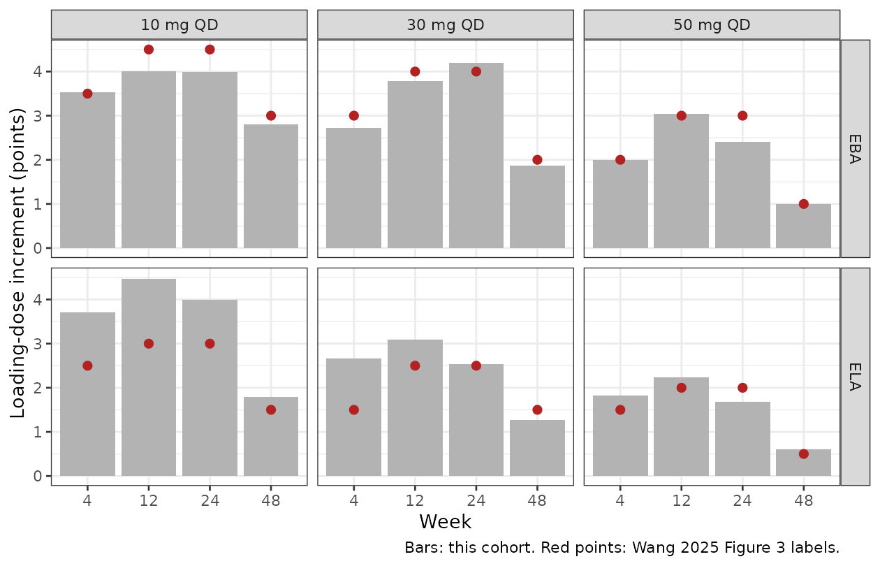
Replicates Figure 3 of Wang 2025.
fig3 %>%
  dplyr::mutate(dplyr::across(c(loading, noLoading, simulated), ~ round(.x, 1))) %>%
  dplyr::rename(Endpoint = endpoint, `Maintenance (mg QD)` = dose, Week = week,
                `With loading (%)` = loading, `Without loading (%)` = noLoading,
                `Increment (points)` = simulated,
                `Published increment (points)` = published) %>%
knitr::kable(caption = "Loading-dose increments in responder rate: Wang 2025 Figure 3 versus this cohort.")| Endpoint | Maintenance (mg QD) | Week | Published increment (points) | With loading (%) | Without loading (%) | Increment (points) |
|---|---|---|---|---|---|---|
| EBA | 10 | 4 | 3.5 | 5.1 | 1.6 | 3.5 |
| EBA | 10 | 12 | 4.5 | 7.9 | 3.9 | 4.0 |
| EBA | 10 | 24 | 4.5 | 13.1 | 9.1 | 4.0 |
| EBA | 10 | 48 | 3.0 | 21.1 | 18.3 | 2.8 |
| EBA | 30 | 4 | 3.0 | 5.1 | 2.4 | 2.7 |
| EBA | 30 | 12 | 4.0 | 12.4 | 8.7 | 3.8 |
| EBA | 30 | 24 | 4.0 | 26.4 | 22.2 | 4.2 |
| EBA | 30 | 48 | 2.0 | 41.7 | 39.9 | 1.9 |
| EBA | 50 | 4 | 2.0 | 5.1 | 3.1 | 2.0 |
| EBA | 50 | 12 | 3.0 | 16.1 | 13.0 | 3.0 |
| EBA | 50 | 24 | 3.0 | 35.1 | 32.7 | 2.4 |
| EBA | 50 | 48 | 1.0 | 52.8 | 51.8 | 1.0 |
| ELA | 10 | 4 | 2.5 | 5.2 | 1.5 | 3.7 |
| ELA | 10 | 12 | 3.0 | 8.2 | 3.8 | 4.5 |
| ELA | 10 | 24 | 3.0 | 13.2 | 9.2 | 4.0 |
| ELA | 10 | 48 | 1.5 | 19.5 | 17.7 | 1.8 |
| ELA | 30 | 4 | 1.5 | 5.2 | 2.5 | 2.7 |
| ELA | 30 | 12 | 2.5 | 13.6 | 10.5 | 3.1 |
| ELA | 30 | 24 | 2.5 | 25.0 | 22.4 | 2.5 |
| ELA | 30 | 48 | 1.5 | 38.5 | 37.2 | 1.3 |
| ELA | 50 | 4 | 1.5 | 5.2 | 3.3 | 1.8 |
| ELA | 50 | 12 | 2.0 | 16.8 | 14.6 | 2.2 |
| ELA | 50 | 24 | 2.0 | 32.2 | 30.5 | 1.7 |
| ELA | 50 | 48 | 0.5 | 47.4 | 46.8 | 0.6 |
stopifnot(
  # The loading dose always helps (paired cohort, monotone model).
  all(fig3$simulated > 0),
  # Agreement with the published increments.
  median(abs(fig3$simulated - fig3$published)) < 1.5,
  # Section 3.3: the loading dose adds more for EBA than for ELA.
  sum(fig3$simulated[fig3$endpoint == "EBA"]) >
    sum(fig3$simulated[fig3$endpoint == "ELA"])
)
Score-category time course
The expected share of each score over 48 weeks for the cohort under placebo, 10 mg, 50 mg and 200/50 mg QD – the quantity the paper’s VPCs (Figures S6 and S8) display, here as a model prediction rather than a VPC.
catTime <- dplyr::bind_rows(
  doseSims[["EBA 0"]] %>% dplyr::mutate(endpoint = "EBA", regimen = "Placebo"),
  doseSims[["EBA 10"]] %>% dplyr::mutate(endpoint = "EBA", regimen = "10 mg"),
  doseSims[["EBA 50"]] %>% dplyr::mutate(endpoint = "EBA", regimen = "50 mg"),
  loadSims[["EBA 50"]] %>% dplyr::mutate(endpoint = "EBA", regimen = "200/50 mg"),
  doseSims[["ELA 0"]] %>% dplyr::mutate(endpoint = "ELA", regimen = "Placebo"),
  doseSims[["ELA 10"]] %>% dplyr::mutate(endpoint = "ELA", regimen = "10 mg"),
  doseSims[["ELA 50"]] %>% dplyr::mutate(endpoint = "ELA", regimen = "50 mg"),
  loadSims[["ELA 50"]] %>% dplyr::mutate(endpoint = "ELA", regimen = "200/50 mg")
) %>%
  dplyr::group_by(endpoint, regimen, time) %>%
  dplyr::summarise(dplyr::across(c(p0, p1, p2, p3), mean), .groups = "drop") %>%
  tidyr::pivot_longer(c(p0, p1, p2, p3), names_to = "score",
                      values_to = "probability") %>%
  dplyr::mutate(
    score = sub("p", "Score ", score),
    regimen = factor(regimen, c("Placebo", "10 mg", "50 mg", "200/50 mg"))
  )

ggplot(catTime, aes(time, 100 * probability, colour = regimen)) +
  geom_line() +
  facet_grid(score ~ endpoint) +
  labs(x = "Week", y = "Expected share of participants (%)", colour = "Regimen") +
  theme_bw()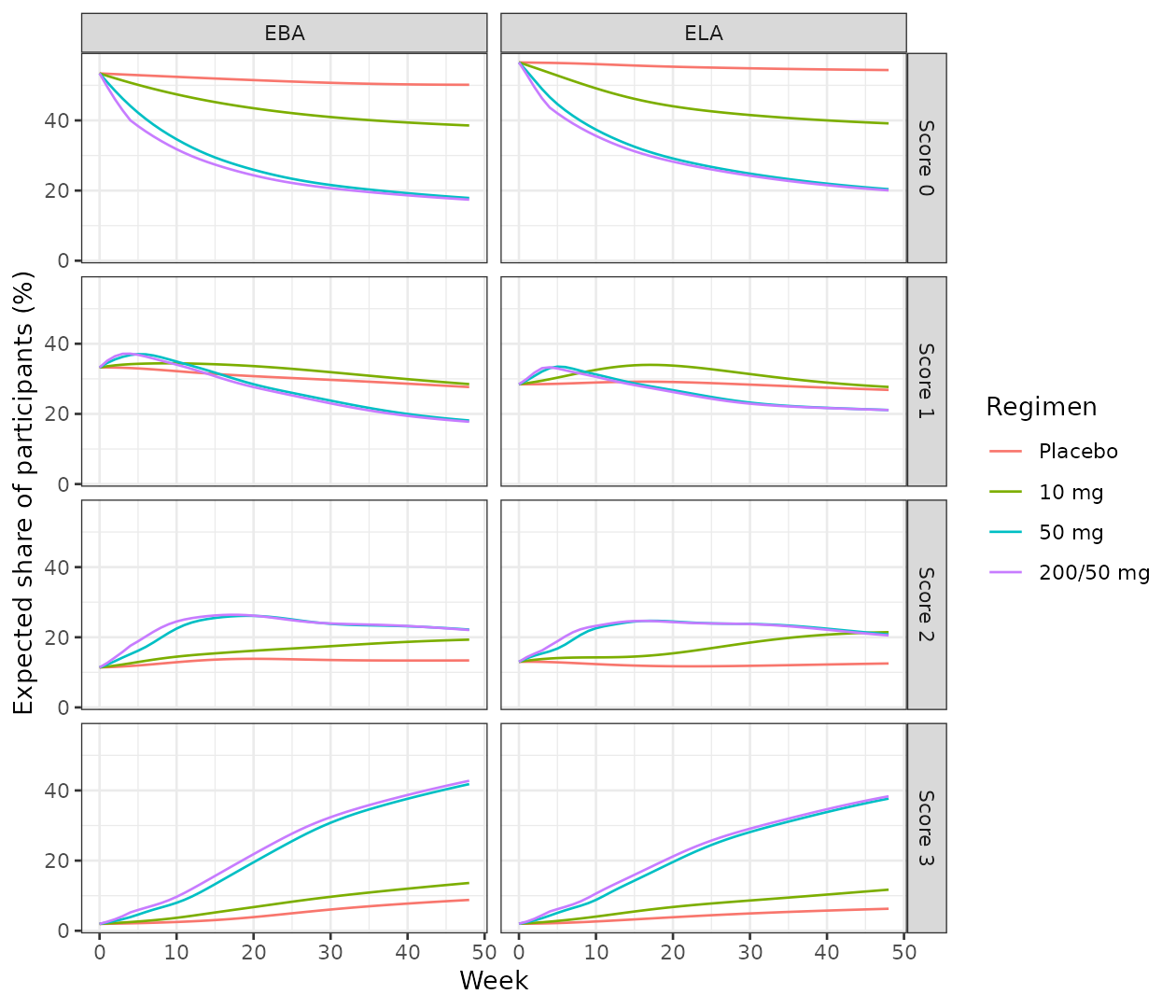
To simulate individual scores rather than probabilities, solve with
the models’ own random effects; the ordinal endpoint is drawn into the
sim column, where category k is score
k - 1:
# Illustration only: rxode2's stream differs across thread counts, so no
# assertion is made on these draws.
rxode2::rxSetSeed(20250214)
draws <- rxode2::rxSolve(
  eba,
  makeEvents(data.frame(from = 0, cav = cavOf(50)),
             data.frame(id = 1:20, RACE_ASIAN = 0L), weeks = c(0, 24, 48)),
  returnType = "data.frame"
)
#> ℹ parameter labels from comments will be replaced by 'label()'
table(week = draws$time, score = draws$sim - 1)
#>     score
#> week  0  1  2  3
#>   0  12  7  1  0
#>   24  5  6  8  1
#>   48  5  2  5  8
Assumptions and deviations
-
Sign of the drug effect in Eq 4. Eq 3-4 of the
paper print
alpha_j + Drug Effect + Placebo Effect, which would make the drug raise the cumulative probability of low scores, i.e. worsen eyebrows and eyelashes. Both control streams instead computeB1 + PBOEFF - DEEFF, and the published responder simulations (Figures 2 and 3, reproduced above) are only recovered with the drug effect subtracted. The models follow the control streams. The placebo term keeps the printed+sign; because the typicalPmaxis zero and its random effect is symmetric, that sign does not change any population prediction. -
B2andB3are log-scale. Tables 3 and 4 label the rows “Difference in baselines”, but the control streams setB2 = EXP(THETA(2))andB3 = EXP(THETA(3)), and the tabulated asymptotic CIs are symmetric around the estimate, as they are on the THETA scale. The baseline-distribution check above confirms it: read as linear gaps, the cut-offs put 94% of participants at score 0 against 55% observed. -
Placebo effect solved in closed form. The ELA
control stream integrates the placebo latent variable as a second
compartment (
dA_pbo/dt = -k A_pbo,A_pbo(0) = 1); the EBA stream uses its exact solutionexp(-k t). Both packaged models use the exact solution. -
Time unit. The control streams run in hours and
convert the half-life with
log(2)/(168 * THETA(6)); the packaged models run in weeks withk = log(2)/thalfrec_drug. - Exposure in the simulations. The paper used individual empirical-Bayes PK for each simulated participant and 4-week average Cavg. This vignette uses the typical-value steady-state Cavg of the packaged PK model for every participant, which omits between-subject PK variability. Ritlecitinib reaches steady state within a day (half-life about 2 hours), so a 4-week average and the steady-state Cavg coincide except across the loading-to-maintenance step.
- Simulated cohort. One cohort of 200 participants per model replaces the paper’s 1000 trials of 200; the comparison is with the published medians. Expected responder rates are computed from the per-participant score probabilities rather than from drawn scores.
-
Not modelled as covariates. Age, sex (eyebrow
model) and geographic region were screened but not retained (Section
2.3.3); they are recorded in
covariatesDataExcluded.