Recombinant Erwinia chrysanthemi asparaginase in healthy adults (Lin 2021)
Source:vignettes/articles/Lin_2021_asparaginaseErwiniaRecombinant.Rmd
Lin_2021_asparaginaseErwiniaRecombinant.Rmd
mod <- rxode2::rxode(readModelDb("Lin_2021_asparaginaseErwiniaRecombinant"))
#> ℹ parameter labels from comments will be replaced by 'label()'
Model and source
- Citation: Lin T, Dumas T, Kaullen J, Berry NS, Choi MR, Zomorodi K, Silverman JA. Population pharmacokinetic model development and simulation for recombinant Erwinia asparaginase produced in Pseudomonas fluorescens (JZP-458). Clin Pharmacol Drug Dev. 2021;10(12):1503-1513. doi:10.1002/cpdd.1002
- Description: One-compartment population PK model for recombinant Erwinia chrysanthemi asparaginase (JZP-458, marketed as Rylaze) given intramuscularly or as a 2-hour intravenous infusion to healthy adults (Lin 2021, phase 1 study JZP458-101). The measured quantity is serum asparaginase activity (SAA), so all amounts are activity units (IU) rather than mass. Intravenous doses enter the central compartment directly. Intramuscular doses use sequential mixed-order absorption: the bioavailable fraction F enters the depot as a zero-order input at a constant rate R1 while first-order absorption ka drains the depot into the central compartment, which makes the terminal phase absorption rate limited (flip-flop) after intramuscular dosing. Body weight is an allometric (power) covariate on clearance; interindividual variability is exponential on clearance and volume, with a proportional residual error.
- Article: https://doi.org/10.1002/cpdd.1002
- Later patient model that reused this paper’s absorption structure:
Lin_2023_asparaginaseErwiniaRecombinant(doi:10.1111/cts.13499).
JZP-458 (marketed as Rylaze) is a recombinant Erwinia chrysanthemi asparaginase produced in a Pseudomonas fluorescens expression platform. It is given to patients with acute lymphoblastic leukemia (ALL) or lymphoblastic lymphoma (LBL) who have developed hypersensitivity to E. coli-derived asparaginases. The measured quantity is serum asparaginase activity (SAA), and the therapeutic target is a nadir SAA (NSAA) of at least 0.1 IU/mL.
This phase 1 model was fit jointly to intramuscular (IM) and intravenous (IV) data, so – unlike the later patient model – it estimates the IM bioavailability relative to IV and the IV volume and clearance directly.
Population
The model was fit to 331 quantifiable SAA observations from 24 healthy adults in the phase 1, single-center, open-label study JZP458-101 (Miami, Florida, November 2018 to May 2019). Participants received a single dose of JZP-458 at 12.5 or 25 mg/m^2 IM, or 25 or 37.5 mg/m^2 as a 2-hour IV infusion (six per arm), with intensive sampling to 96 h. Mean (SD) age was 38.3 (8.6) years, weight 78.3 (9.6) kg and body surface area 1.9 (0.1) m^2; 71% were male, 83% White and 17% Black/African American, and 96% Hispanic/Latino (Lin 2021 Table 1).
str(mod$population, max.level = 1)
#> List of 13
#>  $ species       : chr "human"
#>  $ n_subjects    : int 24
#>  $ n_studies     : int 1
#>  $ n_observations: int 331
#>  $ age_range     : chr "18-55 years (eligibility); mean 38.3 +/- 8.6 years"
#>  $ weight_range  : chr "mean 78.3 +/- 9.6 kg"
#>  $ bsa_range     : chr "mean 1.9 +/- 0.1 m^2"
#>  $ sex_female_pct: num 29.2
#>  $ race_ethnicity: Named num [1:3] 83 17 96
#>   ..- attr(*, "names")= chr [1:3] "White" "Black/African American" "Hispanic/Latino"
#>  $ disease_state : chr "Healthy adult volunteers (body mass index 19.0-30.0 kg/m^2)."
#>  $ dose_range    : chr "Single dose of JZP-458: 12.5 or 25 mg/m^2 intramuscular (n = 6 each; dorsogluteal or deltoid, at most 2 mL per "| __truncated__
#>  $ regions       : chr "United States (single center, Miami, Florida)"
#>  $ notes         : chr "Lin 2021 Methods (Study design) and Table 1. Phase 1, randomized, single-center, open-label study JZP458-101 (N"| __truncated__
Source trace
Every ini() entry in
inst/modeldb/specificDrugs/Lin_2021_asparaginaseErwiniaRecombinant.R
carries an in-file comment naming its origin. They are collected here
for review.
| Equation / parameter | Value | Source location |
|---|---|---|
lcl (CL, 70 kg) |
146 mL/h | Lin 2021 Table 2 (95% CI 128.4-163.6, RSE 6.15%); Results final CL equation |
e_wt_cl |
0.863 | Lin 2021 Table 2 CL row 146 x (WT/70)^0.863; Results
final CL equation |
lvc (Vd) |
3030 mL | Lin 2021 Table 2 (95% CI 2655-3405, RSE 6.32%) |
lfdepot (F, IM) |
0.365 | Lin 2021 Table 2 (95% CI 0.3074-0.4226, RSE 8.05%); Results “bioavailability at 36.5%” |
lka (ka) |
0.0348 1/h | Lin 2021 Table 2 (95% CI 0.02942-0.04018, RSE 7.89%) |
lr1 (zero-order input) |
4000 IU/h | Lin 2021 Table 2 (95% CI 1569-6431, RSE 31.01%) |
etalcl |
0.03502 (BSV 18.88%) | Lin 2021 Table 2 BSV% column, log(1 + 0.1888^2)
|
etalvc |
0.09783 (BSV 32.06%) | Lin 2021 Table 2 BSV% column, log(1 + 0.3206^2)
|
propSd |
0.206 | Lin 2021 Table 2 “Error model proportional 20.6%” |
| One compartment, linear elimination | n/a | Lin 2021 Results, Base model and final covariate model |
| Sequential mixed-order IM absorption | n/a | Lin 2021 Results, Base model |
| IM-only bioavailability relative to IV | n/a | Lin 2021 Results, Base model; Table 2 footnote |
| Exponential BSV, allometric weight on CL | n/a | Lin 2021 Table 2 footnotes |
| IV infusion duration 2 h | n/a | Lin 2021 Methods, Study design |
Model structure
IV doses enter central directly. IM doses enter
depot with sequential mixed-order
absorption: the bioavailable fraction F * amt
fills the depot as a zero-order input at the constant rate
R1, while first-order absorption ka drains the
depot into central at the same time. R1 is the
NONMEM reserved zero-order input rate for the dosing compartment, so the
input duration is F * amt / R1; the same encoding is used
by the later Lin_2023_asparaginaseErwiniaRecombinant
model.
After IV dosing the terminal slope reports
kel = CL / Vd; after IM dosing ka (0.0348 /h)
is smaller than kel (0.048 /h for a 70 kg adult), so the IM
terminal phase is absorption rate limited (flip-flop). This is why Lin
2021 reports a half-life only for the IV route.
Intramuscular dose records must set rate = -1
rxode2 only consults a modelled rate() when the dose
record asks for it. With the default rate = 0 the modelled
rate is silently ignored and the IM dose becomes an instantaneous bolus
into the depot. The check below confirms that, with
rate = -1, the depot fills for exactly
F * amt / R1 hours.
tv <- rxode2::zeroRe(mod)
theta <- mod$theta
cl70 <- exp(theta[["lcl"]])
v_i <- exp(theta[["lvc"]])
f_i <- exp(theta[["lfdepot"]])
ka_i <- exp(theta[["lka"]])
r1_i <- exp(theta[["lr1"]])

# Typical-value single-dose solve. route = "IM" doses the depot with the
# modelled zero-order rate; route = "IV" is a 2-hour infusion into central.
solve_one <- function(dose, route, wt = 70, times = seq(0, 240, by = 0.25),
                      im_rate = -1) {
  ev <- if (route == "IM") {
    rxode2::et(amt = dose, cmt = "depot", rate = im_rate)
  } else {
    rxode2::et(amt = dose, cmt = "central", dur = 2)
  }
  ev <- rxode2::et(ev, times, cmt = "central")
  ev <- as.data.frame(ev)
  ev$WT <- wt
  out <- rxode2::rxSolve(tv, ev, returnType = "data.frame",
                         rtol = 1e-10, atol = 1e-12)
  if (is.null(out$id)) out$id <- 1L
  out[!is.na(out$Cc), ]
}

probe_dose <- 30000   # IU; see "Dose units" below
s_im <- solve_one(probe_dose, "IM", times = seq(0, 240, by = 0.05))
#> ℹ omega/sigma items treated as zero: 'etalcl', 'etalvc'
s_im_bolus <- solve_one(probe_dose, "IM", times = seq(0, 240, by = 0.05),
                        im_rate = 0)
#> ℹ omega/sigma items treated as zero: 'etalcl', 'etalvc'
dur_expected <- f_i * probe_dose / r1_i

rate_check <- data.frame(
  Quantity = c("depot peak time (h)", "Tmax of Cc (h)", "Cmax (IU/mL)"),
  `rate = -1` = c(s_im$time[which.max(s_im$depot)],
                  s_im$time[which.max(s_im$Cc)], max(s_im$Cc)),
  `rate = 0` = c(s_im_bolus$time[which.max(s_im_bolus$depot)],
                 s_im_bolus$time[which.max(s_im_bolus$Cc)],
                 max(s_im_bolus$Cc)),
  check.names = FALSE
)
knitr::kable(rate_check, digits = 3,
caption = "The modelled zero-order rate is active only with rate = -1.")| Quantity | rate = -1 | rate = 0 |
|---|---|---|
| depot peak time (h) | 2.750 | 0.00 |
| Tmax of Cc (h) | 25.700 | 24.30 |
| Cmax (IU/mL) | 1.119 | 1.12 |
Dose units: activity units, not mass
The model’s amount unit is IU of asparaginase activity, not
mg. The zero-order absorption rate is reported in IU/h (Lin
2021 Table 2) and Cc = central / vc is IU/mL only if
central holds IU. Lin 2021 doses in mg/m^2 but does not
state the mg-to-IU specific activity of JZP-458, so dose this
model in IU; no conversion factor is built into the model
file.
The checks in the next three sections use only dose-independent quantities. A reconstruction of the dose scale from the paper’s own simulation table follows them and is labelled as such.
Validation 1: derived quantities printed in Table 2
The Table 2 footnotes print the apparent IM clearance and volume for
a 70 kg adult (CL/F = 0.4 L/h, Vd/F = 8.30 L)
and the IV half-life (t1/2 = ln(2) / (CL / Vd) = 14.4 h).
All three follow from the ini() values by arithmetic, and
the half-life is also recovered from a simulated IV profile.
s_iv <- solve_one(probe_dose, "IV")
#> ℹ omega/sigma items treated as zero: 'etalcl', 'etalvc'
tail_iv <- s_iv[s_iv$time >= 24 & s_iv$time <= 96, ]
thalf_iv_sim <- log(2) /
  -stats::coef(stats::lm(log(tail_iv$Cc) ~ tail_iv$time))[[2]]

derived <- data.frame(
  Quantity = c("CL/F, 70 kg (L/h)", "Vd/F (L)", "IV t1/2 (h), arithmetic",
               "IV t1/2 (h), simulated terminal slope"),
  Model = c(cl70 / f_i / 1000, v_i / f_i / 1000, log(2) * v_i / cl70,
            thalf_iv_sim),
  Published = c(0.4, 8.30, 14.4, 14.4)
)
derived$`Difference (%)` <- 100 * (derived$Model - derived$Published) /
  derived$Published
knitr::kable(derived, digits = 3,
caption = "Model versus the derived values printed in Lin 2021 Table 2.")| Quantity | Model | Published | Difference (%) |
|---|---|---|---|
| CL/F, 70 kg (L/h) | 0.400 | 0.4 | 0.000 |
| Vd/F (L) | 8.301 | 8.3 | 0.017 |
| IV t1/2 (h), arithmetic | 14.385 | 14.4 | -0.103 |
| IV t1/2 (h), simulated terminal slope | 14.385 | 14.4 | -0.103 |
Validation 2: exact bioavailability and weight identities
Elimination is linear, so the IM-to-IV AUC ratio at equal dose must
equal F, and halving body weight must raise AUC by
2^0.863 (AUC = dose / CL, with CL proportional
to WT^0.863).
auc_of <- function(s) {
  sum(diff(s$time) * (utils::head(s$Cc, -1) + utils::tail(s$Cc, -1)) / 2)
}
grid_long <- seq(0, 1500, by = 0.25)
auc_iv70 <- auc_of(solve_one(probe_dose, "IV", times = grid_long))
#> ℹ omega/sigma items treated as zero: 'etalcl', 'etalvc'
auc_im70 <- auc_of(solve_one(probe_dose, "IM", times = grid_long))
#> ℹ omega/sigma items treated as zero: 'etalcl', 'etalvc'
auc_iv35 <- auc_of(solve_one(probe_dose, "IV", wt = 35, times = grid_long))
#> ℹ omega/sigma items treated as zero: 'etalcl', 'etalvc'

id_check <- data.frame(
  Comparison = c("AUC IM / AUC IV (= F)", "AUC IV 35 kg / 70 kg (= 2^0.863)",
                 "AUC IV x CL / dose (= 1)"),
  Observed = c(auc_im70 / auc_iv70, auc_iv35 / auc_iv70,
               auc_iv70 * cl70 / probe_dose),
  Expected = c(0.365, 2^0.863, 1)
)
knitr::kable(id_check, digits = 5,
caption = "Exposure identities reproduce F and the weight exponent.")| Comparison | Observed | Expected |
|---|---|---|
| AUC IM / AUC IV (= F) | 0.36500 | 0.36500 |
| AUC IV 35 kg / 70 kg (= 2^0.863) | 1.81882 | 1.81882 |
| AUC IV x CL / dose (= 1) | 1.00000 | 1.00000 |
Validation 3: PKNCA on typical single-dose profiles
NCA is run on the typical-value (no IIV, no residual error)
single-dose profile for each route, at the 70 kg reference weight to
which Table 2’s half-life refers. Lin 2021 reports a half-life for the
IV route only; the IM terminal phase is absorption rate limited and
reports ln(2) / ka.
nca_sim <- dplyr::bind_rows(
  dplyr::mutate(solve_one(probe_dose, "IV", wt = 70), treatment = "IV"),
  dplyr::mutate(solve_one(probe_dose, "IM", wt = 70), treatment = "IM")
) |>
  dplyr::filter(!is.na(Cc)) |>
  dplyr::select(id, treatment, time, Cc) |>
  dplyr::mutate(Cc = pmax(Cc, 0)) |>
  dplyr::group_by(treatment) |>
  dplyr::filter(time <= time[which.max(Cc)] | Cc >= 1e-6 * max(Cc)) |>
  dplyr::ungroup()
#> ℹ omega/sigma items treated as zero: 'etalcl', 'etalvc'
#> ℹ omega/sigma items treated as zero: 'etalcl', 'etalvc'
stopifnot(all(nca_sim$time[!duplicated(nca_sim$treatment)] == 0))

dose_df <- data.frame(id = 1L, treatment = c("IV", "IM"), time = 0,
                      amt = probe_dose)
o_conc <- PKNCA::PKNCAconc(nca_sim, Cc ~ time | treatment + id)
o_dose <- PKNCA::PKNCAdose(dose_df, amt ~ time | treatment + id)
o_data <- PKNCA::PKNCAdata(
  o_conc, o_dose,
  intervals = data.frame(start = 0, end = 240, cmax = TRUE, tmax = TRUE,
                         half.life = TRUE, auclast = TRUE)
)
nca_res <- as.data.frame(PKNCA::pk.nca(o_data))
nca_res |>
  dplyr::filter(PPTESTCD %in% c("cmax", "tmax", "half.life", "auclast")) |>
  dplyr::select(treatment, PPTESTCD, PPORRES) |>
  tidyr::pivot_wider(names_from = PPTESTCD, values_from = PPORRES) |>
  dplyr::rename("Route" = treatment, "Cmax (IU/mL)" = cmax, "Tmax (h)" = tmax,
                "t1/2 (h)" = half.life, "AUC0-240 (IU*h/mL)" = auclast) |>
  knitr::kable(digits = 3,
caption = "PKNCA on the typical single-dose profile (30000 IU probe dose).")| Route | AUC0-240 (IU*h/mL) | Cmax (IU/mL) | Tmax (h) | t1/2 (h) |
|---|---|---|---|---|
| IM | 74.935 | 1.119 | 25.75 | 20.789 |
| IV | 205.475 | 9.439 | 2.00 | 14.385 |
hl <- nca_res |> dplyr::filter(PPTESTCD == "half.life")
stopifnot(nrow(hl) == 2L)
simulated <- data.frame(treatment = hl$treatment, PPTESTCD = "half.life",
                        PPORRES = hl$PPORRES)
reference <- data.frame(treatment = "IV", half.life = 14.4)
knitr::kable(
  nlmixr2lib::ncaComparisonTable(simulated, reference, by = "treatment",
                                 units = c(half.life = "h")),
  caption = "Typical-value IV half-life versus Lin 2021 Table 2."
)| NCA parameter | treatment | Reference | Simulated | % diff |
|---|---|---|---|---|
| t½ (h) | IV | 14.4 | 14.4 | -0.1% |
hl_iv <- hl$PPORRES[hl$treatment == "IV"]
hl_im <- hl$PPORRES[hl$treatment == "IM"]
stopifnot(
  abs(hl_iv - 14.4) / 14.4 < 0.02,
  abs(hl_im - log(2) / ka_i) / (log(2) / ka_i) < 0.05
)
At the phase 1 mean weight of 78.3 kg the IV half-life would be
shorter, 13.1 h, because CL scales with weight while
Vd does not.
Validation 4: the Table 3 simulation summary
Lin 2021 Table 3 reports, for adult and pediatric virtual populations (1000 each, drawn from NHANES), the mean SAA and the percentage of participants with SAA at or above 0.1 IU/mL at three times on a Monday/Wednesday/Friday schedule (doses at 0, 48, 96, 168, 216 and 264 h): 72 h after dose 3 (t = 168 h), 48 h after dose 5 (t = 264 h) and 72 h after dose 6 (t = 336 h).
Virtual cohorts
The NHANES records are not published, so the cohorts are approximated: 200 adults per arm (18-85 years, weight log-normal around 80 kg, height normal around 168 cm) and 200 children per arm (2-17 years, weight and height drawn around age-specific CDC median growth values). BSA, which sets the mg/m^2 dose, uses the Mosteller formula; the paper does not name a BSA formula.
set.seed(2021)
n_per_arm <- 200
cdc_age <- c(2, 4, 6, 8, 10, 12, 14, 16, 17)
wt_med <- stats::approxfun(cdc_age, c(12.5, 16.3, 20.7, 25.6, 32, 40.5, 50, 58, 61),
                           rule = 2)
ht_med <- stats::approxfun(cdc_age, c(87, 102, 116, 128, 138, 150, 162, 169, 171),
                           rule = 2)
make_pop <- function(pop, n) {
  if (pop == "Adults") {
    wt <- stats::rlnorm(n, log(80), 0.22)
    ht <- stats::rnorm(n, 168, 10)
  } else {
    age <- stats::runif(n, 2, 17.99)
    wt <- wt_med(age) * stats::rlnorm(n, 0, 0.2)
    ht <- ht_med(age) * stats::rlnorm(n, 0, 0.04)
  }
  data.frame(pop = pop, WT = wt, BSA = sqrt(wt * ht / 3600))
}
regimens <- data.frame(
  regimen = c("12.5 mg/m^2 IM", "25 mg/m^2 IM", "25 mg/m^2 IV", "37.5 mg/m^2 IV"),
  mgm2 = c(12.5, 25, 25, 37.5),
  route = c("IM", "IM", "IV", "IV")
)
cohort <- tidyr::expand_grid(regimens, pop = c("Adults", "Pediatrics")) |>
  dplyr::group_by(regimen, pop) |>
  dplyr::group_modify(~ dplyr::bind_cols(.x, make_pop(.y$pop, n_per_arm)) |>
                        dplyr::select(-pop)) |>
  dplyr::ungroup() |>
  dplyr::mutate(id = dplyr::row_number())

cohort |>
  dplyr::group_by(pop) |>
  dplyr::summarise(`Median WT (kg)` = stats::median(WT),
                   `Median BSA (m^2)` = stats::median(BSA), .groups = "drop") |>
  dplyr::rename("Population" = pop) |>
knitr::kable(digits = 2, caption = "Virtual cohort body size (per population).")| Population | Median WT (kg) | Median BSA (m^2) |
|---|---|---|
| Adults | 78.59 | 1.91 |
| Pediatrics | 32.61 | 1.13 |
Simulation at a unit dose scale
Because the model is linear in dose, the cohort is simulated with the
dose entered as mg/m^2 x BSA numerically (one model unit
per mg). Every concentration then scales by the same unknown specific
activity k (IU/mg).
dose_times <- c(0, 48, 96, 168, 216, 264)
obs_times <- seq(0, 336, by = 2)
ev_cohort <- lapply(seq_len(nrow(cohort)), function(i) {
  amt <- cohort$mgm2[i] * cohort$BSA[i]
  dose <- if (cohort$route[i] == "IM") {
    data.frame(time = dose_times, amt = amt, cmt = "depot", rate = -1, evid = 1L)
  } else {
    data.frame(time = dose_times, amt = amt, cmt = "central", rate = amt / 2,
               evid = 1L)
  }
  obs <- data.frame(time = obs_times, amt = 0, cmt = "central", rate = 0,
                    evid = 0L)
  e <- rbind(dose, obs)
  e$id <- cohort$id[i]
  e$WT <- cohort$WT[i]
  e
}) |>
  dplyr::bind_rows() |>
  dplyr::arrange(id, time, dplyr::desc(evid))

rxode2::rxSetSeed(2021)
sim <- rxode2::rxSolve(mod, ev_cohort, returnType = "data.frame")
stopifnot(!anyNA(sim$Cc))
sim <- dplyr::left_join(sim, dplyr::select(cohort, id, regimen, pop), by = "id")
Dose-scale reconstruction (not a published value)
k is calibrated on a single Table 3 cell – the adult
37.5 mg/m^2 IV mean SAA 48 h after dose 5 (1.6 IU/mL, the largest adult
mean and so the one with the smallest relative rounding error). The
other 11 adult mean-SAA cells and all 12 adult percentage cells are
held out.
calib <- sim |>
  dplyr::filter(regimen == "37.5 mg/m^2 IV", pop == "Adults", time == 264)
k_iu_per_mg <- 1.6 / mean(calib$Cc)
sprintf("reconstructed specific activity ~ %.0f IU/mg (NOT a published value)",
        k_iu_per_mg)
#> [1] "reconstructed specific activity ~ 647 IU/mg (NOT a published value)"
sim$SAA <- sim$Cc * k_iu_per_mg
landmarks <- data.frame(
  time = c(168, 264, 336),
  landmark = c("Dose 3 72-Hour", "Dose 5 48-Hour", "Dose 6 72-Hour")
)
published <- tibble::tribble(
  ~regimen, ~pop, ~landmark, ~pct_pub, ~mean_pub,
  "12.5 mg/m^2 IM", "Adults", "Dose 3 72-Hour", 99.5, 0.3,
  "12.5 mg/m^2 IM", "Adults", "Dose 5 48-Hour", 100.0, 0.5,
  "12.5 mg/m^2 IM", "Adults", "Dose 6 72-Hour", 99.5, 0.3,
  "12.5 mg/m^2 IM", "Pediatrics", "Dose 3 72-Hour", 99.9, 0.4,
  "12.5 mg/m^2 IM", "Pediatrics", "Dose 5 48-Hour", 100.0, 0.6,
  "12.5 mg/m^2 IM", "Pediatrics", "Dose 6 72-Hour", 99.9, 0.5,
  "25 mg/m^2 IM", "Adults", "Dose 3 72-Hour", 100.0, 0.6,
  "25 mg/m^2 IM", "Adults", "Dose 5 48-Hour", 100.0, 1.0,
  "25 mg/m^2 IM", "Adults", "Dose 6 72-Hour", 100.0, 0.6,
  "25 mg/m^2 IM", "Pediatrics", "Dose 3 72-Hour", 100.0, 0.9,
  "25 mg/m^2 IM", "Pediatrics", "Dose 5 48-Hour", 100.0, 1.3,
  "25 mg/m^2 IM", "Pediatrics", "Dose 6 72-Hour", 100.0, 0.9,
  "25 mg/m^2 IV", "Adults", "Dose 3 72-Hour", 74.5, 0.4,
  "25 mg/m^2 IV", "Adults", "Dose 5 48-Hour", 95.3, 1.1,
  "25 mg/m^2 IV", "Adults", "Dose 6 72-Hour", 74.5, 0.4,
  "25 mg/m^2 IV", "Pediatrics", "Dose 3 72-Hour", 91.7, 1.2,
  "25 mg/m^2 IV", "Pediatrics", "Dose 5 48-Hour", 99.2, 2.1,
  "25 mg/m^2 IV", "Pediatrics", "Dose 6 72-Hour", 91.7, 1.3,
  "37.5 mg/m^2 IV", "Adults", "Dose 3 72-Hour", 80.9, 0.6,
  "37.5 mg/m^2 IV", "Adults", "Dose 5 48-Hour", 97.4, 1.6,
  "37.5 mg/m^2 IV", "Adults", "Dose 6 72-Hour", 80.9, 0.6,
  "37.5 mg/m^2 IV", "Pediatrics", "Dose 3 72-Hour", 94.5, 1.8,
  "37.5 mg/m^2 IV", "Pediatrics", "Dose 5 48-Hour", 99.5, 3.2,
  "37.5 mg/m^2 IV", "Pediatrics", "Dose 6 72-Hour", 94.5, 2.0
)
tab3 <- sim |>
  dplyr::inner_join(landmarks, by = "time") |>
  dplyr::group_by(regimen, pop, landmark) |>
  dplyr::summarise(pct_sim = 100 * mean(SAA >= 0.1), mean_sim = mean(SAA),
                   .groups = "drop") |>
  dplyr::inner_join(published, by = c("regimen", "pop", "landmark")) |>
  dplyr::mutate(calibration = regimen == "37.5 mg/m^2 IV" & pop == "Adults" &
                  landmark == "Dose 5 48-Hour")
stopifnot(nrow(tab3) == 24L)

tab3 |>
  dplyr::select(regimen, pop, landmark, pct_pub, pct_sim, mean_pub, mean_sim,
                calibration) |>
  dplyr::rename("Dose/route" = regimen, "Population" = pop, "Time" = landmark,
                "% >= 0.1 (Lin 2021)" = pct_pub, "% >= 0.1 (model)" = pct_sim,
                "Mean SAA (Lin 2021)" = mean_pub, "Mean SAA (model)" = mean_sim,
                "Calibration cell" = calibration) |>
  knitr::kable(digits = 2,
caption = "Replicates Lin 2021 Table 3 (mean SAA in IU/mL).")| Dose/route | Population | Time | % >= 0.1 (Lin 2021) | % >= 0.1 (model) | Mean SAA (Lin 2021) | Mean SAA (model) | Calibration cell |
|---|---|---|---|---|---|---|---|
| 12.5 mg/m^2 IM | Adults | Dose 3 72-Hour | 99.5 | 100.0 | 0.3 | 0.30 | FALSE |
| 12.5 mg/m^2 IM | Adults | Dose 5 48-Hour | 100.0 | 100.0 | 0.5 | 0.53 | FALSE |
| 12.5 mg/m^2 IM | Adults | Dose 6 72-Hour | 99.5 | 100.0 | 0.3 | 0.30 | FALSE |
| 12.5 mg/m^2 IM | Pediatrics | Dose 3 72-Hour | 99.9 | 100.0 | 0.4 | 0.49 | FALSE |
| 12.5 mg/m^2 IM | Pediatrics | Dose 5 48-Hour | 100.0 | 100.0 | 0.6 | 0.71 | FALSE |
| 12.5 mg/m^2 IM | Pediatrics | Dose 6 72-Hour | 99.9 | 100.0 | 0.5 | 0.53 | FALSE |
| 25 mg/m^2 IM | Adults | Dose 3 72-Hour | 100.0 | 100.0 | 0.6 | 0.58 | FALSE |
| 25 mg/m^2 IM | Adults | Dose 5 48-Hour | 100.0 | 100.0 | 1.0 | 1.02 | FALSE |
| 25 mg/m^2 IM | Adults | Dose 6 72-Hour | 100.0 | 100.0 | 0.6 | 0.59 | FALSE |
| 25 mg/m^2 IM | Pediatrics | Dose 3 72-Hour | 100.0 | 100.0 | 0.9 | 0.98 | FALSE |
| 25 mg/m^2 IM | Pediatrics | Dose 5 48-Hour | 100.0 | 100.0 | 1.3 | 1.41 | FALSE |
| 25 mg/m^2 IM | Pediatrics | Dose 6 72-Hour | 100.0 | 100.0 | 0.9 | 1.05 | FALSE |
| 25 mg/m^2 IV | Adults | Dose 3 72-Hour | 74.5 | 72.5 | 0.4 | 0.38 | FALSE |
| 25 mg/m^2 IV | Adults | Dose 5 48-Hour | 95.3 | 97.0 | 1.1 | 1.02 | FALSE |
| 25 mg/m^2 IV | Adults | Dose 6 72-Hour | 74.5 | 72.5 | 0.4 | 0.39 | FALSE |
| 25 mg/m^2 IV | Pediatrics | Dose 3 72-Hour | 91.7 | 97.5 | 1.2 | 1.60 | FALSE |
| 25 mg/m^2 IV | Pediatrics | Dose 5 48-Hour | 99.2 | 100.0 | 2.1 | 2.65 | FALSE |
| 25 mg/m^2 IV | Pediatrics | Dose 6 72-Hour | 91.7 | 97.5 | 1.3 | 1.74 | FALSE |
| 37.5 mg/m^2 IV | Adults | Dose 3 72-Hour | 80.9 | 81.0 | 0.6 | 0.61 | FALSE |
| 37.5 mg/m^2 IV | Adults | Dose 5 48-Hour | 97.4 | 97.5 | 1.6 | 1.60 | TRUE |
| 37.5 mg/m^2 IV | Adults | Dose 6 72-Hour | 80.9 | 81.0 | 0.6 | 0.61 | FALSE |
| 37.5 mg/m^2 IV | Pediatrics | Dose 3 72-Hour | 94.5 | 98.5 | 1.8 | 2.23 | FALSE |
| 37.5 mg/m^2 IV | Pediatrics | Dose 5 48-Hour | 99.5 | 100.0 | 3.2 | 3.76 | FALSE |
| 37.5 mg/m^2 IV | Pediatrics | Dose 6 72-Hour | 94.5 | 98.5 | 2.0 | 2.39 | FALSE |
adults_held <- dplyr::filter(tab3, pop == "Adults", !calibration)
# Adult held-out cells. The published means are rounded to 0.1 IU/mL and the
# model means carry ~3-4% Monte-Carlo error (200 subjects per arm), as does k.
# Realised max |diff| 0.07 IU/mL; 0.2 still breaks on a mis-transcribed CL, Vd,
# F, ka or R1, each of which moves these troughs by tens of percent.
# Percentages: binomial SE at p = 0.75, n = 200 is ~3 points; 10 is > 3 SE.
stopifnot(
  max(abs(adults_held$mean_sim - adults_held$mean_pub)) < 0.2,
  stats::median(abs(adults_held$mean_sim / adults_held$mean_pub - 1)) < 0.1,
  max(abs(adults_held$pct_sim - adults_held$pct_pub)) < 10
)
Every adult cell is reproduced: the held-out mean SAA values agree to
within the table’s 0.1 IU/mL rounding, and the IV percentages at or
above target (74.5% and 80.9% after dose 3) are matched to within
Monte-Carlo error. Those two IV percentages are sensitive to the IIV
magnitudes as well as to CL, Vd and
k, so they also support the BSV% reading used for
etalcl and etalvc.
Scale-free checks
Two ratios in Table 3 cancel k entirely, so they test
the structural model without the reconstruction: the IM-to-IV mean SAA
ratio at the shared 25 mg/m^2 dose, and the IV trough decay from 48 h to
72 h post dose. Each published ratio is compared against the interval
implied by the table’s 0.1 IU/mL rounding.
mean_of <- function(reg, lm) {
  tab3$mean_sim[tab3$regimen == reg & tab3$pop == "Adults" & tab3$landmark == lm]
}
ratios <- data.frame(
  Ratio = c("IM / IV, 25 mg/m^2, Dose 3 72-Hour",
            "IV 25 mg/m^2, Dose 3 72-Hour / Dose 5 48-Hour"),
  Model = c(mean_of("25 mg/m^2 IM", "Dose 3 72-Hour") /
              mean_of("25 mg/m^2 IV", "Dose 3 72-Hour"),
            mean_of("25 mg/m^2 IV", "Dose 3 72-Hour") /
              mean_of("25 mg/m^2 IV", "Dose 5 48-Hour")),
  Published = c(0.6 / 0.4, 0.4 / 1.1),
  Lower = c(0.55 / 0.45, 0.35 / 1.15),
  Upper = c(0.65 / 0.35, 0.45 / 1.05)
)
knitr::kable(ratios, digits = 3,
caption = "Dose-scale-free ratios versus Lin 2021 Table 3 (adults).")| Ratio | Model | Published | Lower | Upper |
|---|---|---|---|---|
| IM / IV, 25 mg/m^2, Dose 3 72-Hour | 1.511 | 1.500 | 1.222 | 1.857 |
| IV 25 mg/m^2, Dose 3 72-Hour / Dose 5 48-Hour | 0.375 | 0.364 | 0.304 | 0.429 |
Pediatric cells
The pediatric cells are reproduced only qualitatively. The model
gives the paper’s direction and order of magnitude – children reach
higher SAA than adults on the same mg/m^2 dose, most strongly on the IV
route, because Vd has no body-size covariate while the dose
scales with BSA and CL with WT^0.863 – but it
overshoots the published pediatric means by roughly 5-25% on IM and
20-35% on IV. The pediatric cohort here is built from CDC median growth
values, not from the NHANES records the paper resampled, and pediatric
exposure in this model is sensitive to the weight-to-BSA relationship.
The gap is therefore attributed to the cohort, not to the model, but it
is recorded in the Errata rather than gated tightly.
ped <- dplyr::filter(tab3, pop == "Pediatrics")
ped_iv_ratio <- ped$mean_sim[grepl("IV", ped$regimen)] /
  tab3$mean_sim[tab3$pop == "Adults" & grepl("IV", tab3$regimen)]
stopifnot(
  # Children above adults on IV: the model gives ~2.5-4x, far from 1.
  all(ped_iv_ratio > 1.5),
  # Pediatric means within a factor of 1.6 of the published values.
  all(ped$mean_sim / ped$mean_pub > 1 / 1.6 & ped$mean_sim / ped$mean_pub < 1.6),
  all(ped$pct_sim > 85)
)
Figure 4: median SAA with 90% prediction interval
fig4 <- sim |>
  dplyr::group_by(regimen, pop, time) |>
  dplyr::summarise(lo = stats::quantile(SAA, 0.05), med = stats::median(SAA),
                   hi = stats::quantile(SAA, 0.95), .groups = "drop") |>
  dplyr::mutate(panel = paste(regimen, "-", pop),
                lo = pmax(lo, 1e-3))

ggplot2::ggplot(fig4, ggplot2::aes(time)) +
  ggplot2::geom_ribbon(ggplot2::aes(ymin = lo, ymax = hi), alpha = 0.3,
                       fill = "steelblue") +
  ggplot2::geom_line(ggplot2::aes(y = med), colour = "steelblue",
                     linetype = "dashed") +
  ggplot2::geom_hline(yintercept = 0.1, linetype = "dashed") +
  ggplot2::scale_y_log10(limits = c(0.005, 30)) +
  ggplot2::scale_x_continuous(breaks = seq(0, 288, by = 72)) +
  ggplot2::facet_wrap(~panel, nrow = 2) +
  ggplot2::labs(x = "Time (hours)", y = "SAA (IU/mL)",
                caption = paste("Replicates Figure 4 of Lin 2021, using the",
                                "reconstructed dose scale.")) +
  ggplot2::theme_bw(base_size = 8)
#> Warning in ggplot2::scale_y_log10(limits = c(0.005, 30)): log-10 transformation introduced infinite values.
#> log-10 transformation introduced infinite values.
#> Warning: Removed 8 rows containing missing values or values outside the scale range
#> (`geom_ribbon()`).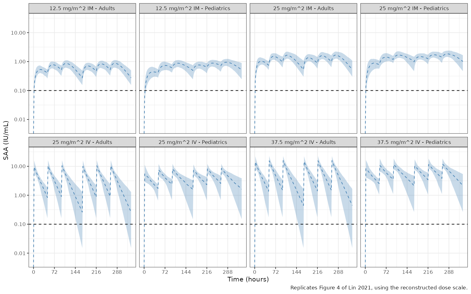
The reconstructed specific activity can be compared with the
independent reconstruction in the
Lin_2023_asparaginaseErwiniaRecombinant article, which
calibrated the later patient model to a figure of that paper and landed
near 580 IU/mg. The two agree to within the precision either can
claim.
stopifnot(k_iu_per_mg > 450, k_iu_per_mg < 900)Assumptions and deviations / Errata
The model’s amount unit is IU, and no mg-to-IU conversion is published. The zero-order absorption rate is reported in IU/h and
Cc = central / vcis IU/mL only if the dose is in IU. Lin 2021 doses in mg/m^2 but does not state the specific activity of JZP-458. Dose this model in IU. No conversion factor is present in the model file.The dose scale used for the Table 3 and Figure 4 replications is reconstructed, not published. It is calibrated on one Table 3 cell and implies about 650 IU/mg. It then reproduces the 11 held-out adult mean-SAA cells and 12 adult percentage cells, and two dose-scale-free ratios confirm the structural model independently of it.
BSV% read as a coefficient of variation. Table 2 prints
BSV%of 18.88 (CL) and 32.06 (Vd) and states that BSV was exponential. These are converted withomega^2 = log(1 + CV^2)(0.03502 and 0.09783). Reading the column as100 * omegainstead would give 0.03565 and 0.1028; at these magnitudes the two readings differ by under 5% in variance and cannot be separated by the published results. No CL-Vd covariance is reported, so the etas are uncorrelated.The weight exponent is encoded as estimated. 0.863 appears only inside the CL row of Table 2 and in the printed final CL equation, with no separate RSE or CI. It is not a conventional value such as 0.75 and the Methods describe weight as a covariate retained by the OFV-drop criterion, so it is not wrapped in
fixed().Absorption structure inferred from prose plus the parameter set. Lin 2021 describes “a sequential mixed order absorption function” estimating “both zero- and first-order absorption rate constant parameters” and reports a zero-order rate in IU/h, but prints no absorption equation. The encoding – the bioavailable dose filling the depot at
R1whilekadrains it – uses exactly the reportedka,R1andF, matches NONMEM’s reservedR1semantics, and is the same encoding as the later Lin 2023 patient model.IV infusion duration. The IV doses are 2-hour infusions (Lin 2021 Methods, Study design), encoded as
dur = 2/rate = amt / 2on records intocentral. The bioavailabilityFapplies to the IM depot only.Virtual cohorts approximate NHANES. The paper resampled 2000 NHANES subjects (1000 adults, 1000 aged 2-17 years); those records are not published. The cohorts here (200 per arm and population) use simple distributional approximations and the Mosteller BSA formula, which the paper does not name. The pediatric cohort is the likely cause of the 5-35% overshoot of the published pediatric means (see “Pediatric cells”).
Ccis the individual prediction, without residual error. Table 3’s percentages may include residual error in the paper’s simulation; the adult percentages are matched within Monte-Carlo error without it.Table 2 parameter differences from the Lin 2023 patient model. Lin 2023 reports
ka0.0369 1/h, zero-order rate 1810 IU/h andF0.359 as fixed from “a PopPK model developed with intensive phase I data”. Those values differ from this paper’s Table 2 (0.0348 1/h, 4000 IU/h, 0.365). This model uses the values printed here.Screened-but-not-retained covariates are documented, not modelled. BSA (significant but not chosen over weight), age, sex and race are recorded in the model file’s
covariatesDataExcludedlist.