Elinzanetant (Willmann 2024)
Source:vignettes/articles/Willmann_2024_elinzanetant.Rmd
Willmann_2024_elinzanetant.RmdModel and source
ui <- rxode2::rxode(readModelDb("Willmann_2024_elinzanetant"))
#> ℹ parameter labels from comments will be replaced by 'label()'
#> Warning: some etas defaulted to non-mu referenced, possible parsing error: etalvc
#> as a work-around try putting the mu-referenced expression on a simple line- Citation: Willmann S, Lloyd A, Austin R, Joseph S, Solms A, Zhang Y, Schneider ARP, Frechen S, Schultze-Mosgau MH. Population pharmacokinetic-pharmacodynamic model of elinzanetant based on integrated clinical phase I and II data. CPT Pharmacometrics Syst Pharmacol. 2024;13(12):2137-2149. doi:10.1002/psp4.13226
- Article: https://doi.org/10.1002/psp4.13226
- Supplement (Data S1, model parameterisation equations and Tables S1-S2): https://doi.org/10.1002/psp4.13226
Elinzanetant is a dual neurokinin-1 (NK-1) and neurokinin-3 (NK-3) receptor antagonist developed for moderate-to-severe vasomotor symptoms (VMS) associated with menopause. Willmann 2024 fitted a single joint model to the parent drug, an intravenous stable-isotope tracer, and three principal metabolites, and coupled it to a fixed-EC50 receptor-occupancy layer.
- Description: Joint population PK/PD model for oral elinzanetant, its intravenous [13C5]-labelled tracer, and its three principal metabolites M30/34, M27 and M18/21, built on integrated phase I and II data from healthy volunteers and women with vasomotor symptoms associated with menopause (Willmann 2024). Elinzanetant and the primary metabolites M30/34 and M27 are two-compartment; the secondary metabolite M18/21 is one-compartment. Absorption is first order with a lag time; a high-fat breakfast and the hard-gel capsule formulation modify the absorption rate constant, the lag time and (high-fat breakfast only) the bioavailability. Elinzanetant clearance is split by fixed fractions into formation of M30/34 (0.6) and M27 (0.3), the remaining 0.1 going to unmodelled metabolites; the linear clearances of M30/34 and M27 both form M18/21. Each metabolite carries an additional saturable Michaelis-Menten elimination. All clearances and Vmax terms follow a 24 h cosine circadian modulation anchored on the clock time of the first dose, with a 49.2% relative amplitude for elinzanetant and 22.5% for the metabolites. NK-1 and NK-3 receptor occupancies are derived from the elinzanetant plasma concentration through Emax relationships with fixed EC50 values.
Population
pop <- ui$population
str(pop, max.level = 1, give.attr = FALSE)
#> List of 14
#>  $ species       : chr "human"
#>  $ n_subjects    : num 195
#>  $ n_studies     : num 7
#>  $ age_range     : chr "22-65 years"
#>  $ age_median    : chr "55 years"
#>  $ weight_range  : chr "51-103.6 kg"
#>  $ weight_median : chr "70 kg"
#>  $ height_median : chr "162 cm"
#>  $ bmi_median    : chr "26.8 kg/m2"
#>  $ sex_female_pct: num 92.8
#>  $ race_ethnicity: Named num [1:3] 78.5 19.5 2
#>  $ disease_state : chr "70.3% healthy volunteers, 29.7% women with moderate-to-severe vasomotor symptoms associated with menopause"
#>  $ dose_range    : chr "25-400 mg orally (soft-gel capsule, hard gel capsule and aqueous suspension) plus a 100 ug [13C5]-elinzanetant "| __truncated__
#>  $ notes         : chr "Model-building dataset: 195 subjects in seven phase I studies contributing 8408 elinzanetant PK observations (5"| __truncated__
The model-building dataset pooled 195 subjects from 7 phase I studies (Willmann 2024 Table 1), contributing 8408 elinzanetant PK observations of which 5.7% were below the limit of quantification and were handled with the M3 method. Fifty-two of those subjects also contributed 2020 observations for each of the three metabolites. Baseline demographics are from Table S1: median age 55 years (22-65 years), median weight 70 kg (51-103.6 kg), median height 162 cm, 92.8% female, 78.5% White / 19.5% Black / 2% Other, and 29.7% women with VMS versus 70.3% healthy volunteers.
A further 171 subjects across three phase I/II studies (including 139 women with VMS in SWITCH-1) formed an external validation dataset used only for visual predictive checks; across both datasets 366 subjects were studied, 336 of them female and 197 women with VMS.
Source trace
Every ini() entry in
inst/modeldb/specificDrugs/Willmann_2024_elinzanetant.R
carries an in-file comment naming its source location. The table below
collects them.
| Equation / parameter | Value | Source location |
|---|---|---|
Circadian modulation
P(t) = Pavg * (1 + AMP * cos(2*pi/24 * (t + TFD + theta_SHIFT)))
|
n/a | Equation 1; restated per parameter in Data S1 |
Receptor occupancy RO = Cpls / (Cpls + EC50)
|
n/a | Equation 2 |
Compartment topology, micro-constants
K12, K24, K42, K35, K53, K67, K76, K89, K98, K20, K26, K28, K610, K810, K100
|
n/a | Figure 1 and Data S1 “Information about PopPK model parametrization” |
lcl (elinzanetant CL) |
7.26 L/h | Table 2, CLpop
|
lvc (elinzanetant Vc) |
23.7 L | Table 2, Vcpop
|
lvp (elinzanetant Vp) |
168 L | Table 2, Vp
|
lq (elinzanetant Q) |
6.57 L/h | Table 2, Q
|
lka |
2.37 1/h | Table 2, KaREF
|
ltlag |
0.292 h | Table 2, ALAGREF
|
lfdepot |
0.367 | Table 2, FREF
|
e_fed_highfat_ka |
-0.911 | Table 2, KaFED2
|
e_form_elz_hardgel_ka |
-0.264 | Table 2, KaFORM3
|
e_fed_highfat_tlag |
0.545 | Table 2, ALFED2
|
e_form_elz_hardgel_tlag |
0.548 | Table 2, ALFORM3
|
e_fed_highfat_fdepot |
-0.227 | Table 2, FFED2
|
lcl_m3034, lvc_m3034,
lvp_m3034, lq_m3034
|
4.14 L/h, 3.58 L, 15.6 L, 3.65 L/h | Table 2, CL3034pop / Vc3034 /
Vp3034 / Q3034
|
lvmax_m3034, lkm_m3034
|
24.1 ug/L/h, 7.87 ug/L | Table 2, Vmax3034 / Km3034
|
lcl_m27, lvc_m27, lvp_m27,
lq_m27
|
4.11 L/h, 1.85 L, 40.4 L, 4.45 L/h | Table 2, CL27pop / Vc27 /
Vp27 / Q27
|
lvmax_m27, lkm_m27
|
42.6 ug/L/h, 17.7 ug/L | Table 2, Vmax27 / Km27
|
lcl_m1821, lvc_m1821
|
9.10 L/h, 0.636 L | Table 2, CL1821pop / Vc1821
|
lvmax_m1821, lkm_m1821
|
335 ug/L/h, 45.8 ug/L | Table 2, Vmax18/21 / Km18/21
|
fm_m3034, fm_m27
|
0.6, 0.3 (fixed constants) | Data S1, FMET3034 / FMET27
|
amp_diurnal, amp_diurnal_met
|
0.492, 0.225 | Table 2, AMP / AMPMET
|
shift_diurnal |
8.05 h | Table 2, theta_SHIFT
|
boxcox_lvc |
2.07 | Table 2, lambda
|
lec50_nk1, lec50_nk3
|
0.97 ug/L, 9.7 ug/L (both fixed) | PK/PD modeling section (NK-1 from the PET study, reference 14; NK-3 assumed 10-fold) |
IIV block on etalcl, etalcl_met,
etalvc
|
0.215 / 0.318 / 0.221 variances; 0.224, 0.164, 0.214 covariances | Table 2 OMEGA, ETA(1,1), ETA(2,2),
ETA(3,3), ETA(2,1), ETA(3,1),
ETA(3,2)
|
etalka, etaltlag
|
0.539, 0.0989 | Table 2 OMEGA, ETA(4,4), ETA(5,5)
|
expSd, expSd_c13,
expSd_m3034, expSd_m27,
expSd_m1821
|
sqrt of 0.378, 0.122, 0.106, 0.143, 0.141 | Table 2 SIGMA, EPS(1,1) to EPS(5,5)
|
Structural verification
Two closed-form checks confirm the ODE system, the unit scaling, the bioavailability and the dosing wiring before any population simulation.
Terminal half-life
The paper states an elimination half-life of approximately 35 h (Introduction). For the two-compartment elinzanetant disposition the terminal rate constant is the smaller eigenvalue of the micro-constant system.
th <- setNames(ui$theta, names(ui$theta))
cl <- exp(th[["lcl"]]); vc <- exp(th[["lvc"]])
vp <- exp(th[["lvp"]]); q  <- exp(th[["lq"]])
k10 <- cl / vc; k12 <- q / vc; k21 <- q / vp
a1 <- k10 + k12 + k21
lambda_z <- (a1 - sqrt(a1^2 - 4 * k10 * k21)) / 2
thalf <- log(2) / lambda_z
c(`terminal half-life (h)` = round(thalf, 2), `paper (h)` = 35)
#> terminal half-life (h)              paper (h)
#>                  34.88                  35.00
Mass balance: AUC at steady state with the circadian term switched off
With a constant clearance, AUC(0-24)ss after once-daily
dosing must equal Dose * F / CL exactly. Setting the
circadian amplitudes to zero and solving the full ten-compartment system
recovers that identity, which validates the dose route, the
bioavailability, the mg to ug/L unit bridge
and the split of elinzanetant clearance across K20,
K26 and K28.
ss_events <- function(tfd, grid = 0.05) {
  ev <- rxode2::et(amt = 120, cmt = "depot", ii = 24, addl = 13) |>
    rxode2::et(seq(312, 336, by = grid), cmt = "central")
  d <- as.data.frame(ev)
  d$id <- 1L
  d$dvid <- ifelse(is.na(d$amt), 1L, NA_integer_)
  d$FED_HIGHFAT <- 0
  d$FORM_ELZ_HARDGEL <- 0
  d$T_FIRSTDOSE <- tfd
  d
}
trapz <- function(x, y) sum(diff(x) * (head(y, -1) + tail(y, -1)) / 2)

mod_flat <- ui |> rxode2::ini(amp_diurnal = 0, amp_diurnal_met = 0)
#> ℹ change initial estimate of `amp_diurnal` to `0`
#> ℹ change initial estimate of `amp_diurnal_met` to `0`
flat <- rxode2::rxSolve(mod_flat, ss_events(9), omega = NA,
                        atol = 1e-10, rtol = 1e-10, useLinCmt = FALSE) |>
  as.data.frame() |>
  dplyr::filter(time >= 312)

auc_flat <- trapz(flat$time, flat$Cc)
auc_analytic <- 120 * 1000 * exp(th[["lfdepot"]]) / cl
c(`simulated AUC(0-24)ss (ug*h/L)` = round(auc_flat, 1),
  `Dose * F / CL (ug*h/L)` = round(auc_analytic, 1),
  `relative difference (%)` = round(100 * (auc_flat / auc_analytic - 1), 3))
#> simulated AUC(0-24)ss (ug*h/L)         Dose * F / CL (ug*h/L)
#>                       6062.000                       6066.100
#>        relative difference (%)
#>                         -0.068
The two agree to better than 0.1%, so the structural implementation is exact.
Replicate Figure 2: circadian modulation of clearance
Figure 2 of Willmann 2024 shows the model-estimated clearances against clock time. The cosine reaches its maximum near 16:00 and its minimum near 04:00 for both the parent and the metabolites, with relative amplitudes of 49.2% and 22.5%.
amp <- th[["amp_diurnal"]]; ampm <- th[["amp_diurnal_met"]]
shift <- th[["shift_diurnal"]]
circ <- tidyr::crossing(
  clock = seq(0, 24, by = 0.1),
  analyte = c("Elinzanetant", "Metabolites (M27, M30/34, M18/21)")
) |>
  dplyr::mutate(
    a = ifelse(analyte == "Elinzanetant", amp, ampm),
    factor = 1 + a * cos(2 * pi / 24 * (clock + shift))
  )

extremes <- circ |>
  dplyr::group_by(analyte) |>
  dplyr::summarise(
    `clock time of maximum (h)` = clock[which.max(factor)],
    `clock time of minimum (h)` = clock[which.min(factor)],
    `relative amplitude (%)` = 100 * unique(a),
    .groups = "drop"
  )
knitr::kable(extremes, digits = 1,
caption = "Timing and amplitude of the circadian clearance cosine.")| analyte | clock time of maximum (h) | clock time of minimum (h) | relative amplitude (%) |
|---|---|---|---|
| Elinzanetant | 15.9 | 3.9 | 49.2 |
| Metabolites (M27, M30/34, M18/21) | 15.9 | 3.9 | 22.5 |
ggplot(circ, aes(clock, factor, colour = analyte)) +
  geom_line(linewidth = 0.9) +
  geom_vline(xintercept = c(4, 16), linetype = "dotted") +
  scale_x_continuous(breaks = seq(0, 24, by = 4)) +
  labs(x = "Clock time (h)", y = "Clearance relative to its 24 h average",
       colour = NULL,
       caption = paste("Replicates Figure 2 of Willmann 2024.",
                       "Dotted lines mark 04:00 and 16:00.")) +
  theme(legend.position = "bottom")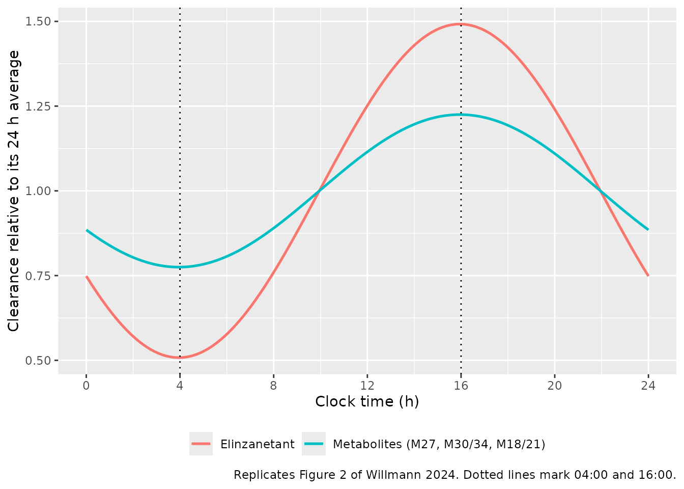
Covariate effects on absorption
The paper reports that a high-fat breakfast decreases Ka by 91%,
increases the absorption lag time by 55% and decreases bioavailability
by 23%, and that the hard gel capsule increases the lag time by 55% and
decreases Ka by 26% (Results and Discussion). The model returns
ka, tlag and fdepot as derived
variables, so the encoded effects can be read back directly.
cov_grid <- tibble::tribble(
  ~scenario,                          ~FED_HIGHFAT, ~FORM_ELZ_HARDGEL,
  "Reference (soft-gel, not high-fat)",          0,                 0,
  "High-fat breakfast",                          1,                 0,
  "Hard gel capsule",                            0,                 1
) |>
  dplyr::mutate(id = dplyr::row_number())

cov_events <- cov_grid |>
  tidyr::crossing(time = c(0, 1)) |>
  dplyr::mutate(
    amt = ifelse(time == 0, 120, NA_real_),
    evid = ifelse(time == 0, 1L, 0L),
    cmt = ifelse(time == 0, "depot", "central"),
    dvid = ifelse(time == 0, NA_integer_, 1L),
    T_FIRSTDOSE = 9
  ) |>
  dplyr::arrange(id, time)

cov_out <- rxode2::rxSolve(ui, cov_events, omega = NA, useLinCmt = FALSE,
                           keep = c("scenario")) |>
  as.data.frame() |>
  dplyr::group_by(scenario) |>
  dplyr::summarise(ka = first(ka), tlag = first(tlag), fdepot = first(fdepot),
                   .groups = "drop")
#> Warning: multi-subject simulation without without 'omega'

ref <- cov_out |> dplyr::filter(scenario == "Reference (soft-gel, not high-fat)")
cov_out |>
  dplyr::mutate(
    `Change in Ka (%)` = 100 * (ka / ref$ka - 1),
    `Change in lag time (%)` = 100 * (tlag / ref$tlag - 1),
    `Change in F (%)` = 100 * (fdepot / ref$fdepot - 1)
  ) |>
  dplyr::rename("Scenario" = scenario, "Ka (1/h)" = ka,
                "Lag time (h)" = tlag, "F (fraction)" = fdepot) |>
  knitr::kable(digits = 3,
               caption = paste("Absorption parameters by feeding and",
                               "formulation scenario. Willmann 2024 reports a",
                               "91% decrease in Ka, a 55% increase in lag time",
                               "and a 23% decrease in F for a high-fat",
                               "breakfast, and a 26% decrease in Ka with a 55%",
"increase in lag time for the hard gel capsule."))| Scenario | Ka (1/h) | Lag time (h) | F (fraction) | Change in Ka (%) | Change in lag time (%) | Change in F (%) |
|---|---|---|---|---|---|---|
| Hard gel capsule | 1.744 | 0.452 | 0.367 | -26.4 | 54.8 | 0.0 |
| High-fat breakfast | 0.211 | 0.451 | 0.284 | -91.1 | 54.5 | -22.7 |
| Reference (soft-gel, not high-fat) | 2.370 | 0.292 | 0.367 | 0.0 | 0.0 | 0.0 |
Virtual cohort
Original observed data are not public. The cohort below mirrors the paper’s steady-state simulation: 1000 virtual women with VMS receiving 120 mg once daily as the soft-gel capsule, dosed either at 09:00 or at 21:00. Two arms of 200 subjects each are used here; 200 per arm is the nlmixr2lib cap and is ample for a 90% prediction interval.
The two arms are paired on identical random effects:
one set of 200 eta vectors is drawn from the model’s OMEGA
and then reused for both dosing times, so the only difference between
the arms is T_FIRSTDOSE. This matters for the ratio
comparison below. Drawing each arm independently would leave the
evening-versus-morning ratios carrying the sampling noise of two
separate 200-subject draws, which for a Cmax whose between-subject CV
exceeds 60% is several percent - comparable to the circadian effect
being measured. Pairing removes that noise entirely, so the ratios
isolate the dosing-time effect. The etas are supplied as explicit
columns and omega = NA is passed to rxSolve(),
which makes the simulation reproducible without relying on rxode2’s
internal sampling order.
set.seed(20241213)
n_per_arm <- 200L

# One shared draw of etas, reused by both arms.
om <- ui$omega
eta_names <- colnames(om)
etas <- matrix(rnorm(n_per_arm * length(eta_names)), nrow = n_per_arm) %*%
  chol(om)
colnames(etas) <- eta_names
etas <- as.data.frame(etas)

make_arm <- function(tfd, label, id_offset = 0L) {
  ev <- rxode2::et(amt = 120, cmt = "depot", ii = 24, addl = 13) |>
    rxode2::et(seq(312, 336, by = 0.25), cmt = "central")
  base <- as.data.frame(ev)
  base$id <- NULL
  base$dvid <- ifelse(is.na(base$amt), 1L, NA_integer_)
  do.call(rbind, lapply(seq_len(n_per_arm), function(i) {
    d <- base
    d$id <- id_offset + i
    d$FED_HIGHFAT <- 0
    d$FORM_ELZ_HARDGEL <- 0
    d$T_FIRSTDOSE <- tfd
    d$regimen <- label
    # subject index, so the paired arms can be matched up afterwards
    d$subject <- i
    for (nm in eta_names) d[[nm]] <- etas[[nm]][i]
    d
  }))
}

events <- dplyr::bind_rows(
  make_arm( 9, "Morning (09:00)", id_offset = 0L),
  make_arm(21, "Evening (21:00)", id_offset = n_per_arm)
)
stopifnot(!anyDuplicated(unique(events[, c("id", "time", "evid")])))
Simulation
sim <- rxode2::rxSolve(ui, events = events,
                       keep = c("regimen", "subject"),
                       omega = NA, useLinCmt = FALSE) |>
  as.data.frame() |>
  dplyr::filter(time >= 312) |>
  dplyr::mutate(
    tad = time - 312,
    clock = (time + T_FIRSTDOSE) %% 24,
    regimen = factor(regimen, levels = c("Morning (09:00)", "Evening (21:00)"))
  )
#> Warning: multi-subject simulation without without 'omega'
stopifnot(nrow(sim) > 0, !anyNA(sim$Cc))
Replicate Figure 4: steady-state profiles and receptor occupancy
pk_band <- sim |>
  dplyr::group_by(regimen, tad) |>
  dplyr::summarise(
    lo = quantile(Cc, 0.05), med = median(Cc), hi = quantile(Cc, 0.95),
    .groups = "drop"
  )

ggplot(pk_band, aes(tad, med)) +
  geom_ribbon(aes(ymin = lo, ymax = hi), fill = "pink", alpha = 0.5) +
  geom_line(linewidth = 0.8) +
  facet_wrap(~regimen) +
  scale_y_log10() +
  scale_x_continuous(breaks = seq(0, 24, by = 6)) +
  labs(x = "Time after dose (h)", y = "Elinzanetant (ug/L)",
       caption = paste("Replicates the upper panels of Figure 4 of",
                       "Willmann 2024: median and 90% prediction interval at",
                       "steady state after 120 mg once daily."))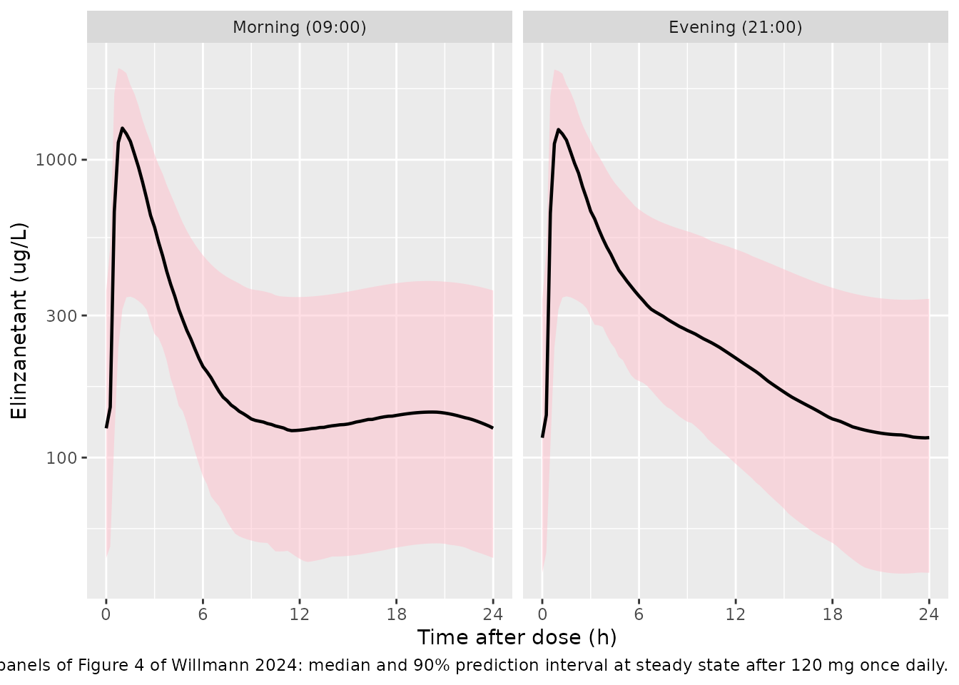
The morning-dosing median profile is non-monotonic: it falls to a
minimum around 11 h after the dose, rises again into the early morning
hours as clearance approaches its 04:00 trough, and then declines to the
pre-dose value. This is the distinctive signature of the circadian
clearance term and is reproduced from the model without any tuning. The
evening-dosing profile is very nearly monotonic by comparison, because
the clearance minimum falls shortly after the dose instead. The paper
quantifies the same contrast as a
Ctrough,ss-versus-Cmin,ss difference of
approximately 9% for morning dosing against approximately 2% for evening
dosing; this implementation returns approximately 6% and approximately
1.5% respectively, reproducing both the direction and the roughly
four-fold asymmetry between the two dosing times (published 4.4-fold,
simulated 4.1-fold).
ro_band <- sim |>
  dplyr::select(regimen, tad, roNK1, roNK3) |>
  tidyr::pivot_longer(c(roNK1, roNK3), names_to = "receptor",
                      values_to = "ro") |>
  dplyr::mutate(receptor = ifelse(receptor == "roNK1", "NK-1", "NK-3")) |>
  dplyr::group_by(regimen, receptor, tad) |>
  dplyr::summarise(
    lo = 100 * quantile(ro, 0.05), med = 100 * median(ro),
    hi = 100 * quantile(ro, 0.95), .groups = "drop"
  )

ggplot(ro_band, aes(tad, med, colour = receptor, fill = receptor)) +
  geom_ribbon(aes(ymin = lo, ymax = hi), alpha = 0.25, colour = NA) +
  geom_line(linewidth = 0.8) +
  facet_wrap(~regimen) +
  coord_cartesian(ylim = c(50, 100)) +
  scale_x_continuous(breaks = seq(0, 24, by = 6)) +
  labs(x = "Time after dose (h)", y = "Receptor occupancy (%)",
       colour = NULL, fill = NULL,
       caption = paste("Replicates the lower panels of Figure 4 of",
                       "Willmann 2024.")) +
  theme(legend.position = "bottom")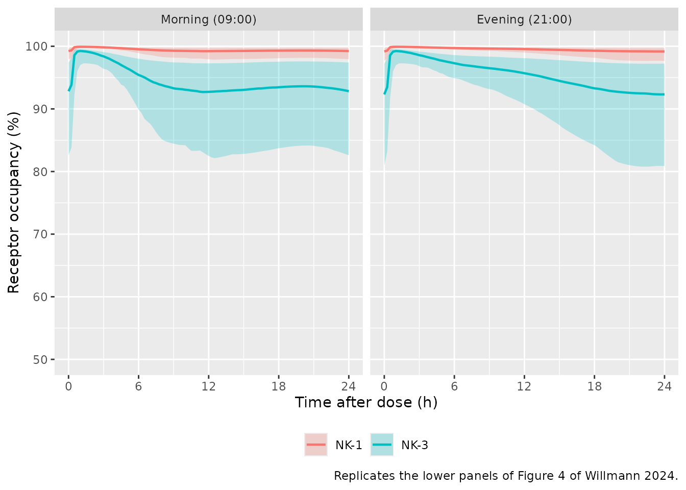
Metabolite profiles
The paper shows metabolite fits only as goodness-of-fit and visual predictive check figures (Figures S3-S10) and reports no numeric metabolite exposures, so this panel is a structural demonstration rather than a numeric validation.
sim |>
  dplyr::select(regimen, tad, Cc, Cc_m3034, Cc_m27, Cc_m1821) |>
  tidyr::pivot_longer(-c(regimen, tad), names_to = "analyte",
                      values_to = "conc") |>
  dplyr::mutate(analyte = factor(
    analyte,
    levels = c("Cc", "Cc_m3034", "Cc_m27", "Cc_m1821"),
    labels = c("Elinzanetant", "M30/34", "M27", "M18/21")
  )) |>
  dplyr::group_by(regimen, analyte, tad) |>
  dplyr::summarise(med = median(conc), .groups = "drop") |>
  ggplot(aes(tad, med, colour = analyte)) +
  geom_line(linewidth = 0.8) +
  facet_wrap(~regimen) +
  scale_y_log10() +
  scale_x_continuous(breaks = seq(0, 24, by = 6)) +
  labs(x = "Time after dose (h)", y = "Median concentration (ug/L)",
       colour = NULL,
       caption = paste("Steady-state median profiles of elinzanetant and its",
                       "three principal metabolites.")) +
  theme(legend.position = "bottom")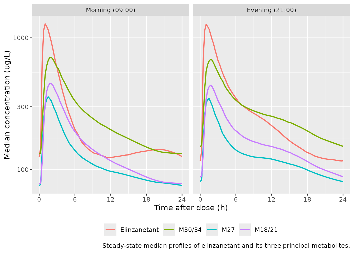
PKNCA validation
The steady-state dosing interval is re-based to 0-24 h. The concentration at time 0 is the steady-state pre-dose trough, not zero, so no zero-concentration anchor row is injected here (that convention applies to single-dose data only).
sim_nca <- sim |>
  dplyr::filter(!is.na(Cc)) |>
  dplyr::select(id, regimen, time = tad, Cc) |>
  dplyr::arrange(id, time)

# Assert the interval anchor exists rather than fabricating it.
stopifnot(all(
  sim_nca |> dplyr::group_by(id) |> dplyr::summarise(has0 = any(time == 0)) |>
    dplyr::pull(has0)
))

conc_obj <- PKNCA::PKNCAconc(sim_nca, Cc ~ time | regimen + id)

dose_df <- sim_nca |>
  dplyr::distinct(id, regimen) |>
  dplyr::mutate(time = 0, amt = 120)
dose_obj <- PKNCA::PKNCAdose(dose_df, amt ~ time | regimen + id)

intervals <- data.frame(
  start = 0, end = 24,
  cmax = TRUE, tmax = TRUE, cmin = TRUE, auclast = TRUE
)

nca_res <- PKNCA::pk.nca(PKNCA::PKNCAdata(conc_obj, dose_obj,
                                          intervals = intervals))
Ctrough,ss in Willmann 2024 Table 3 is the concentration
immediately before the next dose, i.e. the value at 24 h in the re-based
interval. It is computed directly so that it can join the comparison
alongside the PKNCA parameters.
ctrough <- sim_nca |>
  dplyr::filter(time == 24) |>
  dplyr::group_by(regimen) |>
  dplyr::summarise(ctrough = median(Cc), .groups = "drop")
knitr::kable(ctrough, digits = 1,
caption = "Median simulated Ctrough,ss by dosing time.")| regimen | ctrough |
|---|---|
| Morning (09:00) | 125.5 |
| Evening (21:00) | 116.7 |
Comparison against published Table 3
published <- tibble::tribble(
  ~regimen,           ~cmax,  ~cmin, ~auclast,
  "Morning (09:00)",  1534.6, 158.8, 7553.1,
  "Evening (21:00)",  1529.7, 153.7, 8970.0
)

cmp <- nlmixr2lib::ncaComparisonTable(
  simulated = nca_res,
  reference = published,
  by = "regimen",
  params = c("cmax", "cmin", "auclast"),
  units = c(cmax = "ug/L", cmin = "ug/L", auclast = "ug*h/L"),
  tolerance_pct = 20
)

knitr::kable(
  cmp,
  caption = paste("Simulated versus published steady-state exposure",
                  "(Willmann 2024 Table 3, medians of 1000 virtual women",
                  "with VMS). * differs from the reference by more than 20%."),
  align = c("l", "l", "r", "r", "r")
)| NCA parameter | regimen | Reference | Simulated | % diff |
|---|---|---|---|---|
| Cmax (ug/L) | Morning (09:00) | 1530 | 1300 | -15.5% |
| Cmax (ug/L) | Evening (21:00) | 1530 | 1290 | -15.5% |
| Cmin (ug/L) | Morning (09:00) | 159 | 118 | -25.5%* |
| Cmin (ug/L) | Evening (21:00) | 154 | 115 | -25.2%* |
| AUClast (ug*h/L) | Morning (09:00) | 7550 | 5950 | -21.2%* |
| AUClast (ug*h/L) | Evening (21:00) | 8970 | 7280 | -18.8% |
Relative quantities
The absolute exposures run below the published medians (see Errata). The relative quantities in Table 3 - the dosing-time contrasts the paper actually draws its conclusions from - are the more informative check, because they are insensitive to any uniform offset in clearance or bioavailability. Because the two arms are paired on identical etas, these ratios are free of between-arm sampling noise.
All five agree with Table 3 to within 3%, and the
evening-versus-morning Cmax ratio - the one quantity the
paper singles out as showing essentially no dosing-time effect - is
reproduced as 0.997 against a published 0.997. So the circadian
machinery, its phase, and its two amplitudes are all encoded correctly;
what does not reproduce is the absolute exposure level (next
section).
med <- as.data.frame(nca_res) |>
  dplyr::filter(PPTESTCD %in% c("cmax", "cmin", "auclast")) |>
  dplyr::group_by(regimen, PPTESTCD) |>
  dplyr::summarise(v = median(PPORRES), .groups = "drop") |>
  tidyr::pivot_wider(names_from = PPTESTCD, values_from = v) |>
  dplyr::left_join(ctrough, by = "regimen")

get <- function(df, reg, col) df[[col]][df$regimen == reg]
sim_ratio <- c(
  `AUC evening / morning` =
    get(med, "Evening (21:00)", "auclast") / get(med, "Morning (09:00)", "auclast"),
  `Ctrough evening / morning` =
    get(ctrough, "Evening (21:00)", "ctrough") / get(ctrough, "Morning (09:00)", "ctrough"),
  `Cmax evening / morning` =
    get(med, "Evening (21:00)", "cmax") / get(med, "Morning (09:00)", "cmax"),
  `Ctrough / Cmin, morning` =
    get(ctrough, "Morning (09:00)", "ctrough") / get(med, "Morning (09:00)", "cmin"),
  `Ctrough / Cmin, evening` =
    get(ctrough, "Evening (21:00)", "ctrough") / get(med, "Evening (21:00)", "cmin")
)
pub_ratio <- c(8970.0 / 7553.1, 156.7 / 172.7, 1529.7 / 1534.6,
               172.7 / 158.8, 156.7 / 153.7)

tibble::tibble(
  Quantity = names(sim_ratio),
  Simulated = as.numeric(sim_ratio),
  Published = pub_ratio,
  `Difference (%)` = 100 * (as.numeric(sim_ratio) / pub_ratio - 1)
) |>
  knitr::kable(digits = 3,
               caption = paste("Relative steady-state quantities, simulated",
"versus Willmann 2024 Table 3."))| Quantity | Simulated | Published | Difference (%) |
|---|---|---|---|
| AUC evening / morning | 1.223 | 1.188 | 2.998 |
| Ctrough evening / morning | 0.930 | 0.907 | 2.456 |
| Cmax evening / morning | 0.997 | 0.997 | 0.008 |
| Ctrough / Cmin, morning | 1.061 | 1.088 | -2.429 |
| Ctrough / Cmin, evening | 1.015 | 1.020 | -0.470 |
Assumptions and deviations
Errata and discrepancies in the source
-
Table 3 absolute exposures are not reconcilable with the
Table 2 typical values. For once-daily dosing at steady state,
AUC(0-24)ssmust equalDose * F / CLwhenever clearance is constant; with the publishedF = 0.367andCL = 7.26 L/hthat identity gives120000 * 0.367 / 7.26 = 6066 ug*h/L. The published median of7553 ug*h/Lfor morning dosing implies an effective clearance near 5.8 L/h, roughly 20% below the reported typical value, and the evening value of8970 ug*h/Limplies about 4.9 L/h. The circadian term cannot close the gap for morning dosing: with a 09:00 dose the concentration peak sits close to the 16:00 clearance maximum, so the circadian modulation movesAUC(0-24)ssdown relative toDose * F / CL, which is what this implementation reproduces. The mass-balance check above confirms the implementation returns the analytic identity to within 0.1% when the circadian amplitudes are set to zero, so the shortfall is a property of the published numbers rather than of the encoding. Two further observations localise it to the exposure level specifically. First, the shortfall is close to uniform rather than structured: simulatedCmaxis 15.5% below the published median for both dosing times, andCminis 25% below for both, which is the signature of a single multiplicative offset in clearance or bioavailability rather than of a misencoded rate constant. Second, every dosing-time contrast in Table 3 is reproduced to within 3%, including theCmaxevening/morning ratio to three decimal places, so the circadian term and the disposition structure are demonstrably correct. The most likely explanation is that the paper’s 1000 virtual women with VMS were built by resampling individual post-hoc parameter estimates from the female subpopulation rather than by drawing etas around the typical value - the paper describes exactly that resampling procedure for the intrinsic-factor analysis, and male subjects (who had significantly higher metabolite exposure-equivalent clearance) were excluded from the target population. No parameter has been tuned to close the gap. -
Bilirubin covariate direction. The Results and
Discussion prose states that “women with bilirubin levels below the
median were found to have approximately 15% higher elinzanetant
exposure” and that “Low bilirubin levels were associated with a slightly
(approximately 15%) higher elinzanetant exposure”. The Figure 3 forest
plot prints the opposite:
BILI >= median : BILI < median = 1.147 [90% CI 1.063-1.239], i.e. higher bilirubin is associated with roughly 15% higher exposure. The figure’s direction is adopted incovariatesDataExcludedbecause it is the numerically printed result and because it is the direction consistent with the authors’ own mechanistic reading, that the association “might reflect the direct causality between liver function and the hepatic metabolism of elinzanetant”. Bilirubin is not in the final model, so this does not affect any prediction. -
Absorption rate constant unit. The Results text
gives “a first-order absorption rate (Ka) of 2.37 L/h”;
L/his a typographical error for a first-order rate constant. Table 2 gives the unit ash^-1, which is what the model uses. -
Absorption lag time in the Results text. The
Results sentence reads “an absorption lag time of approximately 12.29
a.m.”, which is a typesetting corruption. Table 2 gives
ALAGREF = 0.292 h, which is what the model uses. -
Metabolite circadian amplitude wording. The
Discussion says “for the three metabolites, the relative amplitude was
22.5% smaller”. Table 2 describes
AMPMET = 0.225as the “Amplitude of circadian variation for metabolite clearances and Vmax”, and both the Results sentence (“49.2% and 22.5%, respectively”) and the later Discussion comparison (“49.2% or 22.5%, respectively”) treat 22.5% as the absolute metabolite amplitude. The absolute reading is used.
Modelling assumptions
-
Metabolite formation fractions are encoded as
fixed.
FMET27 = 0.3andFMET3034 = 0.6appear only in Data S1, are described there as “constants”, and carry no standard error or entry in Table 2, so they are wrapped infixed(). The remaining 10% of elinzanetant clearance goes to unmodelled metabolites viaK20. - Both EC50 values are fixed. Neither was estimated in this analysis. The NK-1 value of 0.97 ug/L is carried from the elinzanetant PET study cited as reference 14 (repeated-dosing arm); the NK-3 value of 9.7 ug/L is that value multiplied by ten on the paper’s stated assumption that the in vitro 10-fold affinity difference is maintained in vivo. Receptor occupancy is driven by the elinzanetant plasma concentration alone, as the paper specifies, even though the metabolites are described as pharmacologically similar.
-
Saturable metabolite elimination leaves the system.
Figure 1 draws the
Vmax/Kmarrow from each metabolite’s central compartment to “metabolites”, separately from theK610andK810arrows that form M18/21. The saturable term is therefore an additional elimination pathway, not an alternative route to M18/21. -
The
[13C5]tracer arm is retained. It duplicates the parent disposition parameters but has its own residual error (EPS(2,2)) and its own compartments in Figure 1, and it is what identifies absolute bioavailability. Its metabolites were not measured, so the whole of its clearance leaves the system viaK30. Dose it withcmt = "central_c13". - Mass, not molar, transfer between analytes. The paper’s parameterisation transfers amounts directly between the parent and metabolite compartments with no molecular-weight correction, so the metabolite volumes and clearances are apparent values on the parent’s mass scale. This is replicated as published.
-
Circadian anchor supplied as a covariate. Willmann
2024 Equation 1 writes the cosine argument as
t + TFD + theta_SHIFTwithtthe time since the first dose. The model therefore takes the per-subject clock time of the first dose as the covariateT_FIRSTDOSEand forms wall-clock time internally astime + T_FIRSTDOSE. A time-varying clock-time column cannot be used instead, because the cosine is evaluated inside the ODE at arbitrary solver steps and a 0-24 wrapping covariate cannot be interpolated across midnight. -
Box-Cox IIV on Vc. Data S1 gives
VC = VCpop * exp((exp(eta3)^lambda - 1) / lambda). Becauseexp(eta3)^lambdaequalsexp(lambda * eta3), this is the standard Petersson 2009 Box-Cox eta transformation, and it is implemented in that form. It makesetalvcnon-mu-referenced, which rxode2 reports as a warning when the model is parsed; the warning is expected and does not affect simulation. -
Screened-but-unused covariates. The twelve
intrinsic factors that Willmann 2024 screened post hoc on model-derived
AUC(0-24)ssbut did not retain are documented in the model file’scovariatesDataExcludedlist with their Figure 3 geometric mean ratios and 90% confidence intervals. They are documentation only and are not referenced inmodel(). Vasomotor-symptom patient status (ratio 1.029 [0.954-1.109]) is recorded in the population notes instead, because no canonical covariate column exists for it and it would have required registering one for a documentation-only entry. -
Cohort size and pairing. The paper simulated 1000
virtual women per dosing time; this vignette uses 200 per arm, the
nlmixr2lib cap, which is ample for the 90% prediction intervals shown.
The two arms reuse one shared draw of etas so that the
evening-versus-morning contrasts are paired. With independent draws the
dosing-time ratios are dominated by sampling noise at this cohort size -
the
Cmaxratio moves by more than 10% between independent draws, which is larger than the effect being measured - so pairing is what makes the relative-quantity table above a meaningful check rather than an artefact. -
Provenance comments cannot sit inside the
OMEGAblock. rxode2 rewrites each in-ini()comment to;while parsinglabel()text, which is a syntax error inside the multi-linec()of a correlated-eta block. The six-element lower triangle of the 3x3 block is therefore annotated in a comment block immediately above it rather than element by element.