Piperacillin + tazobactam in Korean patients (Kim 2016)
Source:vignettes/articles/Kim_2016_piperacillin_tazobactam.Rmd
Kim_2016_piperacillin_tazobactam.RmdModel and source
Kim 2016 fitted piperacillin and tazobactam separately, applying the same model-building process to each (“All population pharmacokinetic model processes were equally applied for piperacillin and tazobactam”, Methods section 4) and reporting the two sets of estimates side by side in Table 2. The two fits are therefore packaged as two independent model files, described together here.
ui_pip <- rxode2::rxode(readModelDb("Kim_2016_piperacillin"))
#> ℹ parameter labels from comments will be replaced by 'label()'
ui_taz <- rxode2::rxode(readModelDb("Kim_2016_tazobactam"))
#> ℹ parameter labels from comments will be replaced by 'label()'- Citation: Kim YK, Jung JA, Choi HK, Bae IG, Choi WS, Hur J, Jin SJ, Kim SW, Kwon KT, Lee SR, Shin JG, Kiem S. Population pharmacokinetic analysis of piperacillin/tazobactam in Korean patients with acute infections. Infect Chemother. 2016;48(3):209-215. doi:10.3947/ic.2016.48.3.209. Structural and covariate equations: Results section 2 (‘the final model was as follows’) and the Table 2 structural-model header rows. All parameter estimates: Table 2, piperacillin columns. The a priori linear body-weight adjustment of V1 follows reference [16] of the paper (Li C, Kuti JL, Nightingale CH, Mansfield DL, Dana A, Nicolau DP. J Antimicrob Chemother), cited in Methods section 4. The tazobactam counterpart fitted in the same paper is modellib(‘Kim_2016_tazobactam’).
- Piperacillin model: Two-compartment population PK model for piperacillin in 33 Korean adult inpatients with acute infections (Kim 2016), sampled at steady state after the fourth 1-h IV infusion of 2 g or 4 g piperacillin (with tazobactam) every 8 h. Zero-order IV input into the central compartment, first-order elimination, an additive non-renal-plus-renal clearance linear in Cockcroft-Gault creatinine clearance, and a linear body-weight effect on the central volume; the intercompartmental clearance and the peripheral volume were fixed.
- Tazobactam model: Two-compartment population PK model for tazobactam in 33 Korean adult inpatients with acute infections (Kim 2016), sampled at steady state after the fourth 1-h IV infusion of 0.25 g or 0.5 g tazobactam (with piperacillin) every 8 h. Zero-order IV input into the central compartment, first-order elimination, an additive non-renal-plus-renal clearance linear in Cockcroft-Gault creatinine clearance, and a linear body-weight effect on the central volume; the intercompartmental clearance and the peripheral volume were fixed.
- Article: https://doi.org/10.3947/ic.2016.48.3.209 (open access)
Population
Thirty-three adult inpatients with acute infections were enrolled at six university-affiliated hospitals in Korea between April 2013 and April 2015 (Methods section 1). Thirty-five patients completed the study; two were excluded because sampling at the injection site was suspected – their piperacillin and tazobactam concentrations were roughly 1,000-fold higher than everyone else’s (Results section 1).
The cohort was elderly and renally heterogeneous (Table 1): age 68.79 +/- 10.97 years (range 46-88), body weight 58.17 +/- 10.08 kg (range 36.30-75.40), serum creatinine 1.18 +/- 0.80 mg/dL (range 0.34-4.70) and Cockcroft-Gault creatinine clearance 61.27 +/- 36.67 mL/min (range 14.45-146.01). Seventeen patients (51.5%) were men. Infection sites were lungs (13), urinary tract (12), soft tissue (6) and bloodstream (2). APACHE II score was 13.48 +/- 8.48 (range 3-38) and Glasgow Coma Scale score 13.09 +/- 2.88 (range 7-15).
Dosing followed a renal-function rule (Methods section 2): piperacillin / tazobactam 2 / 0.25 g for creatinine clearance <= 50 mL/min (14 patients, 42.4%) or 4 / 0.5 g for creatinine clearance > 50 mL/min (19 patients, 57.6%), each infused intravenously over 1 h every 8 h for at least four consecutive doses. Blood was drawn at steady state – pre-dose and at 0 min, 30 min and 4-6 h after the end of the fourth infusion.
The same information is available programmatically as
readModelDb("Kim_2016_piperacillin")()$population.
Source trace
Every ini() entry in
inst/modeldb/specificDrugs/Kim_2016_piperacillin.R and
inst/modeldb/specificDrugs/Kim_2016_tazobactam.R carries an
in-file comment naming its source location. They are collected here for
review.
| Equation / parameter | Piperacillin | Tazobactam | Source location |
|---|---|---|---|
| Structural model | 2-compartment, first-order elimination | 2-compartment, first-order elimination | Results sections 2 and 3; Abstract |
TVCL = theta1 + theta5 * CLcr/47 (L/h) |
2.90 + 4.03 * CLcr/47 |
1.76 + 4.81 * CLcr/47 |
Results sections 2 and 3 (“the final model was as follows”); Table 2 structural-model header |
lcl_nonren (theta1, L/h) |
2.90 (RSE 42.41%; bootstrap 2.80, 95% CI 0.01-5.26) | 1.76 (RSE 51.82%; bootstrap 1.72, 95% CI 0.01-3.67) | Table 2 |
lcl_renal (theta5, L/h at CLcr = 47) |
4.03 (RSE 32.75%; bootstrap 3.99, 95% CI 1.82-7.89) | 4.81 (RSE 23.49%; bootstrap 4.79, 95% CI 2.86-7.71) | Table 2 |
TVV1 = theta2 * weight/60 (L) |
19.50 * weight/60 |
22.6 * weight/60 |
Results sections 2 and 3; Table 2 structural-model header |
lvc (theta2, L at 60 kg) |
19.50 (RSE 14.82%; bootstrap 19.31, 95% CI 15.15-29.62) | 22.6 (RSE 10.84%; bootstrap 24.10, 95% CI 20.06-30.79) | Table 2 |
lq (Q, L/h) – fixed |
2.29 (no RSE, no bootstrap) | 1.18 (no RSE, no bootstrap) | Table 2 |
lvp (V2, L) – fixed |
3.76 (no RSE, no bootstrap) | 4.3 (no RSE, no bootstrap) | Table 2 |
crcl_ref (mL/min) |
47 | 47 | Printed in the Table 2 / Results CL equation |
wt_ref (kg) |
60 | 60 | Results sections 2 and 3 (“median body weight of 60 kg”) |
etalcl (omega CL) |
0.279 -> variance 0.077841 | 0.211 -> variance 0.044521 | Table 2, “Random variability (CV,%)” |
etalvc (omega V1) |
0.179 -> variance 0.032041 | 0.151 -> variance 0.022801 | Table 2, “Random variability (CV,%)” |
propSd (sigma, proportional) |
0.399 (RSE 10.78%; bootstrap 0.390, 95% CI 0.297-0.472) | 0.393 (RSE 12.26%; bootstrap 0.387, 95% CI 0.297-0.479) | Table 2, “Residual variability (%)” |
| Residual-error form | proportional only | proportional only | Results sections 2 and 3 |
| IIV distribution | log-normal, independent etas | log-normal, independent etas | Methods section 4 |
| Covariate CLcr on CL | dOFV -10.387 | dOFV -17.736 | Results sections 2 and 3 |
| Covariate weight on V1 | a priori, linear | a priori, linear | Methods section 4 (following the paper’s reference [16]) |
| Input | 1-h zero-order IV infusion into central
|
1-h zero-order IV infusion into central
|
Methods section 2 |
Virtual cohort
The observed concentrations are not publicly available, so a virtual cohort is drawn whose covariate distributions approximate the Table 1 demographics and whose dose assignment follows the study’s renal-function rule exactly.
# set.seed() seeds R's RNG (used for the covariate draw below). It does NOT
# seed rxode2's simulation RNG, whose streams are partitioned per solver
# thread -- so the eta draw differs between a 2-core CI runner and a
# multi-thread workstation. Every assertion downstream is written to hold for
# any cohort this model can produce (see the deterministic gates further down,
# which use zeroRe() and therefore do not depend on the eta draw at all).
set.seed(20160716)

n_per_arm <- 150L

# Truncated normal draw: Table 1 gives mean +/- SD and an observed range for
# each continuous covariate, so values are drawn from the normal and resampled
# until they fall inside the reported range.
rtrunc_norm <- function(n, mean, sd, lo, hi) {
  out <- numeric(0)
  while (length(out) < n) {
    x <- stats::rnorm(n * 4L, mean, sd)
    out <- c(out, x[x >= lo & x <= hi])
  }
  out[seq_len(n)]
}

# Table 1: body weight 58.17 +/- 10.08 kg, range 36.30-75.40.
# Table 1: CLcr 61.27 +/- 36.67 mL/min, range 14.45-146.01. Methods section 2
# splits the cohort at 50 mL/min, so each arm is drawn from its own side of the
# split; this reproduces the protocol and fixes the arm sizes.
make_cohort <- function(n, crcl_lo, crcl_hi, treatment, id_offset = 0L) {
  tibble::tibble(
    id = id_offset + seq_len(n),
    WT = rtrunc_norm(n, 58.17, 10.08, 36.30, 75.40),
    CRCL = rtrunc_norm(n, 61.27, 36.67, crcl_lo, crcl_hi),
    treatment = treatment
  )
}

cohort <- dplyr::bind_rows(
  make_cohort(n_per_arm, 14.45, 50.00, "2/0.25 g q8h (CLcr <= 50)", id_offset = 0L),
  make_cohort(n_per_arm, 50.00, 146.01, "4/0.5 g q8h (CLcr > 50)", id_offset = n_per_arm)
)

stopifnot(
  nrow(cohort) == 2L * n_per_arm,
  !anyDuplicated(cohort$id),
  all(cohort$WT >= 36.30 & cohort$WT <= 75.40),
  all(cohort$CRCL >= 14.45 & cohort$CRCL <= 146.01)
)
The study sampled after the fourth infusion. Eight q8h doses are simulated here instead, so that the last dosing interval is at steady state to within numerical noise even for the slowest-clearing subject; the NCA and the closed-form gates below all run over that last interval.
tau <- 8 # dosing interval (h), Methods section 2
n_doses <- 8L
dose_times <- (seq_len(n_doses) - 1L) * tau
ss_start <- max(dose_times) # start of the final (steady-state) dosing interval
ss_end <- ss_start + tau

# Coarse grid over the approach to steady state, dense grid over the final
# interval so the trapezoidal AUC resolves the 1-h infusion peak.
obs_times <- c(
  seq(0, ss_start - 2, by = 2),
  seq(ss_start, ss_end, by = 0.05)
)

# Piperacillin 2 g / 4 g, tazobactam 0.25 g / 0.5 g (Methods section 2),
# infused over 1 h. `cmt` is the ODE state name on BOTH dose and observation
# rows -- never the algebraic observable `Cc`.
make_events <- function(amt_low, amt_high) {
  doses <- cohort |>
    tidyr::crossing(time = dose_times) |>
    dplyr::mutate(
      evid = 1L,
      cmt = "central",
      amt = ifelse(treatment == "2/0.25 g q8h (CLcr <= 50)", amt_low, amt_high),
      dur = 1
    )
  obs <- cohort |>
    tidyr::crossing(time = obs_times) |>
    dplyr::mutate(evid = 0L, cmt = "central", amt = NA_real_, dur = NA_real_)
  dplyr::bind_rows(doses, obs) |>
    dplyr::arrange(id, time, dplyr::desc(evid))
}

ev_pip <- make_events(2000, 4000)
ev_taz <- make_events(250, 500)

stopifnot(
  !anyDuplicated(unique(ev_pip[, c("id", "time", "evid")])),
  !anyDuplicated(unique(ev_taz[, c("id", "time", "evid")]))
)
Simulation
mod_pip <- readModelDb("Kim_2016_piperacillin")
mod_taz <- readModelDb("Kim_2016_tazobactam")

keep_cols <- c("treatment", "WT", "CRCL")

sim_pip <- rxode2::rxSolve(mod_pip, events = ev_pip, keep = keep_cols) |>
  as.data.frame()
#> ℹ parameter labels from comments will be replaced by 'label()'
sim_taz <- rxode2::rxSolve(mod_taz, events = ev_taz, keep = keep_cols) |>
  as.data.frame()
#> ℹ parameter labels from comments will be replaced by 'label()'

stopifnot(
  nrow(sim_pip) > 0, nrow(sim_taz) > 0,
  all(sim_pip$Cc >= 0, na.rm = TRUE),
  all(sim_taz$Cc >= 0, na.rm = TRUE)
)
A typical-value (between-subject variability removed) companion is
used for the deterministic gates; with zeroRe() each
subject’s clearance is exactly the typical value implied by their own
covariates, so it can be compared against the equation as the paper
prints it.
sim_pip_tv <- rxode2::rxSolve(rxode2::zeroRe(mod_pip), events = ev_pip, keep = keep_cols) |>
  as.data.frame()
#> ℹ parameter labels from comments will be replaced by 'label()'
#> ℹ omega/sigma items treated as zero: 'etalcl', 'etalvc'
#> Warning: multi-subject simulation without without 'omega'
sim_taz_tv <- rxode2::rxSolve(rxode2::zeroRe(mod_taz), events = ev_taz, keep = keep_cols) |>
  as.data.frame()
#> ℹ parameter labels from comments will be replaced by 'label()'
#> ℹ omega/sigma items treated as zero: 'etalcl', 'etalvc'
#> Warning: multi-subject simulation without without 'omega'
Replicate published figures
Kim 2016 Figure 2 is a visual predictive check for the final piperacillin model: 2,000 simulated patients, with the median and the 2.5th / 97.5th predicted percentiles overlaid on the observed concentrations. The observed data are not available here, so the panel below shows the simulated prediction interval only, for the steady-state dosing interval that the study sampled. (Methods section 4 describes the VPC as using 5th / 50th / 95th percentile curves while the Figure 2 caption describes 2.5th / 97.5th; the caption is followed here.)
# Replicates Figure 2 of Kim 2016 (piperacillin VPC), plus the same view for
# tazobactam, over the final steady-state dosing interval.
vpc_band <- function(sim, drug) {
  sim |>
    dplyr::filter(time >= ss_start, time <= ss_end) |>
    dplyr::mutate(tad = time - ss_start, drug = drug) |>
    dplyr::group_by(drug, treatment, tad) |>
    dplyr::summarise(
      Q025 = stats::quantile(Cc, 0.025, na.rm = TRUE),
      Q50 = stats::quantile(Cc, 0.50, na.rm = TRUE),
      Q975 = stats::quantile(Cc, 0.975, na.rm = TRUE),
      .groups = "drop"
    )
}

dplyr::bind_rows(
  vpc_band(sim_pip, "Piperacillin"),
  vpc_band(sim_taz, "Tazobactam")
) |>
  ggplot(aes(tad, Q50)) +
  geom_ribbon(aes(ymin = Q025, ymax = Q975), alpha = 0.25) +
  geom_line() +
  facet_grid(drug ~ treatment, scales = "free_y") +
  labs(
    x = "Time after the start of the steady-state infusion (h)",
    y = "Plasma concentration (mg/L)",
    title = "Steady-state prediction intervals (median, 2.5th-97.5th percentile)",
    caption = "Replicates the simulated bands of Figure 2 of Kim 2016; observed points unavailable."
  ) +
  theme_bw()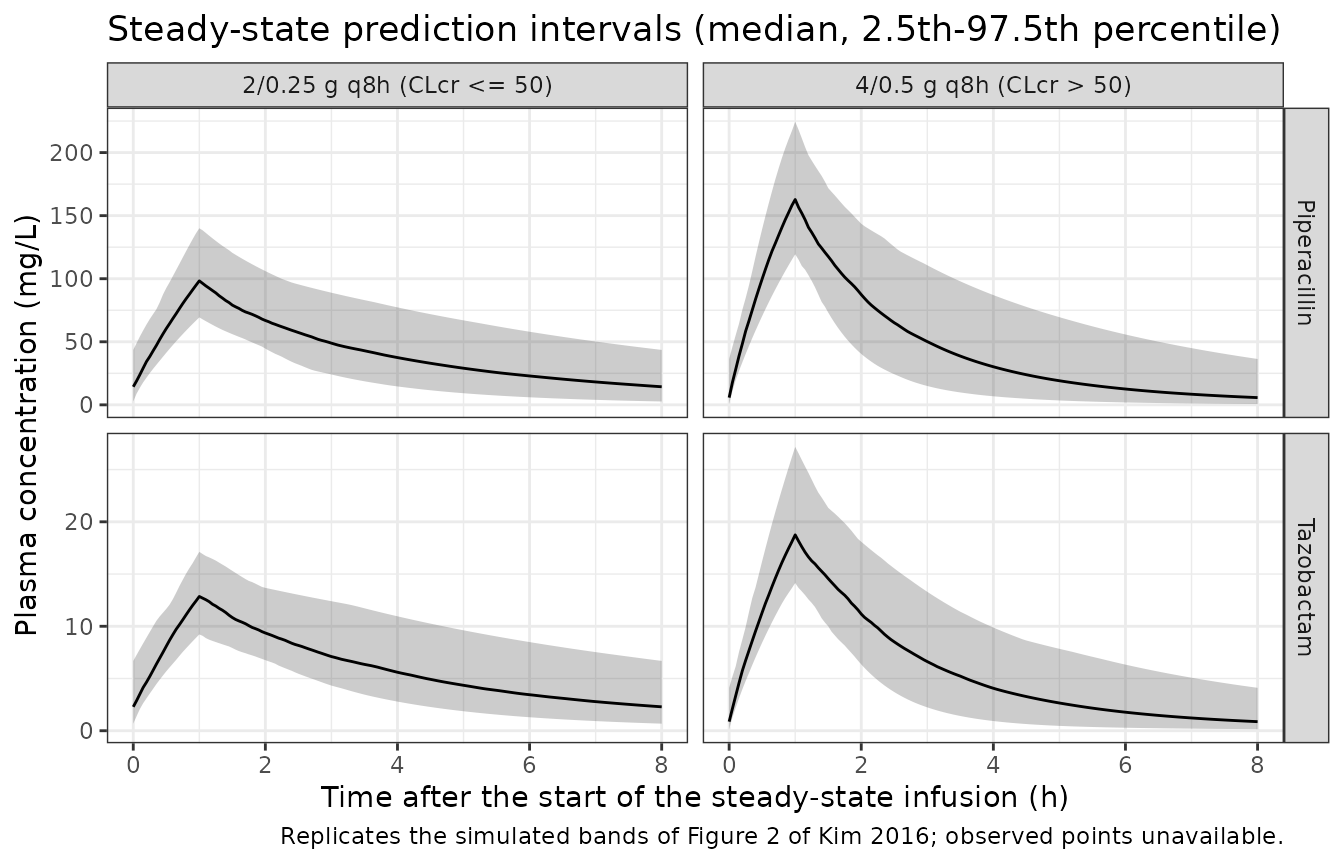
The Discussion contrasts the Korean piperacillin clearance equation
with one developed in Caucasians,
CL = (1.29 * CLcr + 100) * 60/1000 L/h, and concludes that
“clearance of piperacillin in Korean patients is expected to be lower
than that in Caucasians in both normal and lower renal function within
the normal body weight range”. That comparison is reproduced below.
crcl_grid <- seq(14.45, 146.01, length.out = 200)
cl_compare <- dplyr::bind_rows(
  tibble::tibble(
    CRCL = crcl_grid,
    CL = 2.90 + 4.03 * crcl_grid / 47,
    Equation = "Korean (Kim 2016)"
  ),
  tibble::tibble(
    CRCL = crcl_grid,
    CL = (1.29 * crcl_grid + 100) * 60 / 1000,
    Equation = "Caucasian (Kim 2016 Discussion)"
  )
)

ggplot(cl_compare, aes(CRCL, CL, colour = Equation)) +
  geom_line(linewidth = 0.9) +
  labs(
    x = "Creatinine clearance (mL/min)",
    y = "Typical piperacillin CL (L/h)",
    title = "Korean vs Caucasian piperacillin clearance equations",
    caption = "Reproduces the comparison made in the Discussion of Kim 2016."
  ) +
  theme_bw() +
  theme(legend.position = "bottom")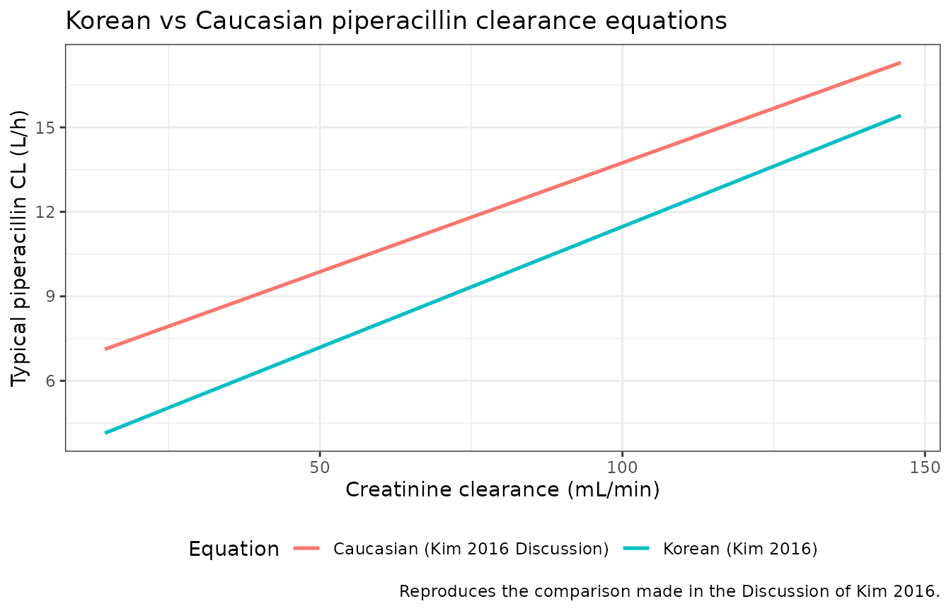
PKNCA validation
NCA is computed over the final steady-state dosing interval, grouped by treatment arm.
# Only `!is.na(Cc)` -- adding `time > 0` or `Cc > 0` would drop the row that
# anchors the AUC interval.
nca_conc <- function(sim) {
  sim |>
    dplyr::filter(!is.na(Cc), time >= ss_start, time <= ss_end) |>
    dplyr::select(id, time, Cc, treatment)
}

nca_dose <- function(ev) {
  ev |>
    dplyr::filter(evid == 1, time == ss_start) |>
    dplyr::select(id, time, amt, treatment)
}

ss_intervals <- data.frame(
  start = ss_start,
  end = ss_end,
  cmax = TRUE,
  tmax = TRUE,
  cmin = TRUE,
  auclast = TRUE,
  cav = TRUE
)

run_nca <- function(sim, ev, concu, doseu) {
  conc_obj <- PKNCA::PKNCAconc(
    nca_conc(sim), Cc ~ time | treatment + id,
    concu = concu, timeu = "h"
  )
  dose_obj <- PKNCA::PKNCAdose(
    nca_dose(ev), amt ~ time | treatment + id,
    doseu = doseu
  )
  PKNCA::pk.nca(PKNCA::PKNCAdata(conc_obj, dose_obj, intervals = ss_intervals))
}

nca_pip <- run_nca(sim_pip, ev_pip, "mg/L", "mg")
nca_taz <- run_nca(sim_taz, ev_taz, "mg/L", "mg")

stopifnot(
  nrow(as.data.frame(nca_pip$result)) > 0,
  nrow(as.data.frame(nca_taz$result)) > 0
)
nca_summary <- function(res, drug) {
  as.data.frame(res$result) |>
    dplyr::filter(PPTESTCD %in% c("cmax", "tmax", "cmin", "auclast", "cav")) |>
    dplyr::group_by(treatment, PPTESTCD) |>
    dplyr::summarise(
      median = stats::median(PPORRES),
      q05 = stats::quantile(PPORRES, 0.05),
      q95 = stats::quantile(PPORRES, 0.95),
      .groups = "drop"
    ) |>
    dplyr::mutate(
      Drug = drug,
      Parameter = nlmixr2lib::ncaParamLabel(PPTESTCD),
      Value = sprintf("%.3g (%.3g, %.3g)", median, q05, q95)
    ) |>
    dplyr::select(Drug, treatment, Parameter, Value)
}

dplyr::bind_rows(
  nca_summary(nca_pip, "Piperacillin"),
  nca_summary(nca_taz, "Tazobactam")
) |>
  dplyr::rename("Dose arm" = treatment) |>
  knitr::kable(
    caption = paste(
      "Simulated steady-state NCA over the final dosing interval:",
      "median (5th, 95th percentile) across 150 subjects per arm.",
      "Concentrations in mg/L, AUC in mg*h/L, times in h."
    )
)| Drug | Dose arm | Parameter | Value |
|---|---|---|---|
| Piperacillin | 2/0.25 g q8h (CLcr <= 50) | AUClast | 334 (207, 554) |
| Piperacillin | 2/0.25 g q8h (CLcr <= 50) | Cavg | 41.8 (25.9, 69.2) |
| Piperacillin | 2/0.25 g q8h (CLcr <= 50) | Cmax | 98.3 (73.7, 135) |
| Piperacillin | 2/0.25 g q8h (CLcr <= 50) | Cmin | 14.3 (3.87, 37.1) |
| Piperacillin | 2/0.25 g q8h (CLcr <= 50) | Tmax | 1 (1, 1) |
| Piperacillin | 4/0.5 g q8h (CLcr > 50) | AUClast | 387 (230, 672) |
| Piperacillin | 4/0.5 g q8h (CLcr > 50) | Cavg | 48.4 (28.7, 84) |
| Piperacillin | 4/0.5 g q8h (CLcr > 50) | Cmax | 163 (124, 217) |
| Piperacillin | 4/0.5 g q8h (CLcr > 50) | Cmin | 5.74 (1.03, 30.4) |
| Piperacillin | 4/0.5 g q8h (CLcr > 50) | Tmax | 1 (1, 1) |
| Tazobactam | 2/0.25 g q8h (CLcr <= 50) | AUClast | 47.6 (32.3, 73) |
| Tazobactam | 2/0.25 g q8h (CLcr <= 50) | Cavg | 5.95 (4.03, 9.13) |
| Tazobactam | 2/0.25 g q8h (CLcr <= 50) | Cmax | 12.9 (9.36, 16.7) |
| Tazobactam | 2/0.25 g q8h (CLcr <= 50) | Cmin | 2.29 (0.882, 5.33) |
| Tazobactam | 2/0.25 g q8h (CLcr <= 50) | Tmax | 1 (1, 1) |
| Tazobactam | 4/0.5 g q8h (CLcr > 50) | AUClast | 48.5 (30.7, 79.1) |
| Tazobactam | 4/0.5 g q8h (CLcr > 50) | Cavg | 6.06 (3.84, 9.89) |
| Tazobactam | 4/0.5 g q8h (CLcr > 50) | Cmax | 18.7 (14.6, 25.6) |
| Tazobactam | 4/0.5 g q8h (CLcr > 50) | Cmin | 0.869 (0.224, 3.51) |
| Tazobactam | 4/0.5 g q8h (CLcr > 50) | Tmax | 1 (1, 1) |
Comparison against published NCA
Kim 2016 reports no non-compartmental parameters –
neither a Cmax / Tmax / AUC / half-life table nor per-arm exposure
summaries. Figure 1 is a goodness-of-fit panel and Figure 2 a visual
predictive check; Table 1 is demographics and Table 2 is model
parameters. There is therefore nothing to put on the reference side of
nlmixr2lib::ncaComparisonTable(), and no such table is
rendered. The closed-form gates below take its place: they check that
the packaged model reproduces the equations the paper does
print, and that the simulated exposures are internally consistent with
them.
Closed-form validation gates
Gate 1 – steady-state AUC reproduces the paper’s printed clearance equation
At steady state, the AUC over one dosing interval satisfies
AUC_tau = Dose / CL exactly, for any linear
multi-compartment model. The clearance implied by the simulated profile
is therefore Dose / AUC_tau, and it must equal the
clearance obtained by evaluating the paper’s printed equation at the
subject’s own creatinine clearance. The equations are transcribed here
directly from Results sections 2 and 3 – independently of how the model
file encodes them – so a mis-transcribed intercept, slope or reference
constant in the model file makes this gate go red.
nca_typical <- function(sim, ev, concu) {
  res <- run_nca(sim, ev, concu, "mg")
  as.data.frame(res$result) |>
    dplyr::filter(PPTESTCD == "auclast") |>
    dplyr::select(id, treatment, auc_tau = PPORRES) |>
    dplyr::left_join(
      ev |>
        dplyr::filter(evid == 1, time == ss_start) |>
        dplyr::select(id, amt, CRCL),
      by = "id"
    ) |>
    dplyr::mutate(cl_from_auc = amt / auc_tau)
}

# Kim 2016 Results section 2: CL (L/h) = 2.9 + 4.03 * CLcr/47
gate1_pip <- nca_typical(sim_pip_tv, ev_pip, "mg/L") |>
  dplyr::mutate(
    cl_from_paper = 2.9 + 4.03 * CRCL / 47,
    pct_diff = 100 * (cl_from_auc - cl_from_paper) / cl_from_paper
  )

# Kim 2016 Results section 3: CL (L/h) = 1.76 + 4.81 * CLcr/47
gate1_taz <- nca_typical(sim_taz_tv, ev_taz, "mg/L") |>
  dplyr::mutate(
    cl_from_paper = 1.76 + 4.81 * CRCL / 47,
    pct_diff = 100 * (cl_from_auc - cl_from_paper) / cl_from_paper
  )

# Deterministic comparison: both sides use the same typical-value parameters,
# so the only difference is trapezoidal error on a 0.05 h grid plus the
# residual approach to steady state after 7 dosing intervals. A tight all()
# bound is correct here (there is no per-subject random mechanism separating
# the two sides), and it goes red on any transcription error in theta1,
# theta5 or the 47 mL/min reference -- each of which moves CL by tens of
# percent.
stopifnot(
  max(abs(gate1_pip$pct_diff)) < 1,
  max(abs(gate1_taz$pct_diff)) < 1
)

tibble::tibble(
  Drug = c("Piperacillin", "Tazobactam"),
  `Max |% difference|` = c(
    max(abs(gate1_pip$pct_diff)),
    max(abs(gate1_taz$pct_diff))
  ),
  `Median |% difference|` = c(
    stats::median(abs(gate1_pip$pct_diff)),
    stats::median(abs(gate1_taz$pct_diff))
  )
) |>
  knitr::kable(
    digits = 4,
    caption = "Gate 1: Dose / AUC_tau at steady state vs the paper's printed CL equation."
)| Drug | Max |% difference| | Median |% difference| |
|---|---|---|
| Piperacillin | 0.0102 | 0.0027 |
| Tazobactam | 0.1875 | 0.0036 |
Gate 2 – central volume reproduces the printed weight relationship
The end-of-infusion concentration of the first dose is not a
clean read on V1 for a two-compartment model, but the model’s own
vc output column is, and it must equal
theta2 * weight/60 evaluated independently from Results
sections 2 and 3. This gate protects the wt_ref = 60
reference and the linear (exponent 1, not allometric 0.75) form.
vc_check <- function(sim_tv, theta2) {
  sim_tv |>
    dplyr::distinct(id, WT, vc) |>
    dplyr::mutate(
      vc_from_paper = theta2 * WT / 60,
      pct_diff = 100 * (vc - vc_from_paper) / vc_from_paper
    )
}

gate2_pip <- vc_check(sim_pip_tv, 19.50)
gate2_taz <- vc_check(sim_taz_tv, 22.6)

stopifnot(
  max(abs(gate2_pip$pct_diff)) < 1e-8,
  max(abs(gate2_taz$pct_diff)) < 1e-8
)

tibble::tibble(
  Drug = c("Piperacillin", "Tazobactam"),
  `V1 at 60 kg (L)` = c(
    unique(round(gate2_pip$vc_from_paper[which.min(abs(gate2_pip$WT - 60))], 2)),
    unique(round(gate2_taz$vc_from_paper[which.min(abs(gate2_taz$WT - 60))], 2))
  ),
  `Max |% difference|` = c(
    max(abs(gate2_pip$pct_diff)),
    max(abs(gate2_taz$pct_diff))
  )
) |>
knitr::kable(caption = "Gate 2: model V1 vs the printed theta2 * weight/60 relationship.")| Drug | V1 at 60 kg (L) | Max |% difference| |
|---|---|---|
| Piperacillin | 19.51 | 0 |
| Tazobactam | 22.61 | 0 |
Gate 3 – terminal half-life reproduces the two-compartment closed form
Q and V2 are not exercised by Gate 1 (steady-state AUC depends only on CL) or Gate 2. They are gated here through the terminal disposition rate constant of the two-compartment system,
beta = 0.5 * ((kel + k12 + k21) - sqrt((kel + k12 + k21)^2 - 4 * kel * k21)),
compared against the PKNCA half-life of a single-dose washout at the
reference subject (60 kg, CLcr 47 mL/min). A wrong Q or V2 changes
beta and the gate goes red.
lambda_z is restricted to 28 h post-dose and later
rather than left to PKNCA’s automatic point selection. For tazobactam
the distribution rate constant (alpha = 0.43 /h) is only
about 2.4-fold faster than beta = 0.18 /h, so an earlier
window still carries distribution-phase curvature and
lambda_z reads steep: PKNCA’s automatic selection began at
13.2 h and returned a half-life of 3.65 h against a closed-form 3.76 h –
a 3.0% bias in the instrument, not in the model.
r.squared does not warn about it; it was 0.9999 on the
biased fit.
The window is set with PKNCAconc(include_half.life = ),
which takes the name of a logical column of the concentration
data. Note that lambda.z.time.first in the
intervals data frame is a reporting flag, not a window
setting – putting a time there is rejected outright.
ref_subject <- tibble::tibble(
  id = 1L, WT = 60, CRCL = 47, treatment = "reference"
)

washout_end <- 40 # h of observation after the single dose
lambda_z_start <- 28 # h; start of the terminal-slope window

washout_events <- function(amt) {
  dplyr::bind_rows(
    ref_subject |> dplyr::mutate(time = 0, evid = 1L, cmt = "central", amt = amt, dur = 1),
    ref_subject |>
      tidyr::crossing(time = seq(0, washout_end, by = 0.05)) |>
      dplyr::mutate(evid = 0L, cmt = "central", amt = NA_real_, dur = NA_real_)
  ) |>
    dplyr::arrange(time, dplyr::desc(evid))
}

half_life_check <- function(mod, amt, theta1, theta5, theta2, q, vp) {
  ev <- washout_events(amt)
  sim <- rxode2::rxSolve(rxode2::zeroRe(mod), events = ev, keep = c("treatment")) |>
    as.data.frame()
  if (is.null(sim$id)) sim$id <- 1L
  stopifnot(all(sim$Cc >= 0, na.rm = TRUE))

  conc <- sim |>
    dplyr::filter(!is.na(Cc)) |>
    dplyr::select(id, time, Cc, treatment) |>
    dplyr::mutate(include_hl = time >= lambda_z_start)
  dose <- ev |>
    dplyr::filter(evid == 1) |>
    dplyr::select(id, time, amt, treatment)

  # The tail is still far above solver noise at 40 h (0.0037 mg/L for
  # piperacillin against a Cmax of 165 mg/L, 0.0056 against 18.8 for
  # tazobactam), so the log-linear fit is not reading rounding error.
  stopifnot(
    sum(conc$include_hl) > 50,
    all(conc$Cc[conc$include_hl] > 1e-4)
  )

  res <- PKNCA::pk.nca(PKNCA::PKNCAdata(
    PKNCA::PKNCAconc(
      conc, Cc ~ time | treatment + id,
      concu = "mg/L", timeu = "h",
      include_half.life = "include_hl"
    ),
    PKNCA::PKNCAdose(dose, amt ~ time | treatment + id, doseu = "mg"),
    intervals = data.frame(start = 0, end = Inf, half.life = TRUE)
  ))
  hl_nca <- as.data.frame(res$result) |>
    dplyr::filter(PPTESTCD == "half.life") |>
    dplyr::pull(PPORRES)

  # Closed form from values transcribed directly from Kim 2016 Table 2.
  cl <- theta1 + theta5 * 47 / 47
  v1 <- theta2 * 60 / 60
  kel <- cl / v1
  k12 <- q / v1
  k21 <- q / vp
  s <- kel + k12 + k21
  beta <- 0.5 * (s - sqrt(s^2 - 4 * kel * k21))
  list(hl_nca = hl_nca, hl_closed = log(2) / beta)
}

gate3_pip <- half_life_check(mod_pip, 4000, 2.90, 4.03, 19.50, 2.29, 3.76)
#> ℹ parameter labels from comments will be replaced by 'label()'
#> ℹ omega/sigma items treated as zero: 'etalcl', 'etalvc'
gate3_taz <- half_life_check(mod_taz, 500, 1.76, 4.81, 22.6, 1.18, 4.3)
#> ℹ parameter labels from comments will be replaced by 'label()'
#> ℹ omega/sigma items treated as zero: 'etalcl', 'etalvc'

gate3 <- tibble::tibble(
  Drug = c("Piperacillin", "Tazobactam"),
  `Closed-form t1/2 (h)` = c(gate3_pip$hl_closed, gate3_taz$hl_closed),
  `PKNCA t1/2 (h)` = c(gate3_pip$hl_nca, gate3_taz$hl_nca)
) |>
  dplyr::mutate(
    `% difference` = 100 * (`PKNCA t1/2 (h)` - `Closed-form t1/2 (h)`) / `Closed-form t1/2 (h)`
  )

# Deterministic: a typical-value solve against its own closed form, with no
# per-subject random mechanism separating the two sides, so a tight bound is
# correct here rather than a cohort-robust one. Realised -0.000% (piperacillin)
# and -0.070% (tazobactam) on the 28-40 h window. 0.5% leaves headroom for
# platform-to-platform solver differences while still going red on a wrong Q or
# V2: halving V2 moves the piperacillin closed-form t1/2 by 16% and doubling Q
# moves it by 7%.
stopifnot(max(abs(gate3$`% difference`)) < 0.5)

knitr::kable(
  gate3,
  digits = 3,
  caption = "Gate 3: PKNCA terminal half-life vs the two-compartment closed form at the reference subject."
)| Drug | Closed-form t1/2 (h) | PKNCA t1/2 (h) | % difference |
|---|---|---|---|
| Piperacillin | 2.616 | 2.616 | 0.000 |
| Tazobactam | 3.764 | 3.761 | -0.071 |
Gate 4 – the Discussion’s Korean-vs-Caucasian clearance claim
gate4 <- tibble::tibble(
  CRCL = c(20, 47, 100, 146),
  `Korean CL (L/h)` = 2.90 + 4.03 * CRCL / 47,
  `Caucasian CL (L/h)` = (1.29 * CRCL + 100) * 60 / 1000
) |>
  dplyr::mutate(`Korean lower?` = `Korean CL (L/h)` < `Caucasian CL (L/h)`)

# The paper's Discussion claim is categorical ("lower ... in both normal and
# lower renal function"), and both equations here are deterministic, so an
# exact comparison is appropriate -- no simulated quantity is involved.
stopifnot(all(gate4$`Korean lower?`))

knitr::kable(
  gate4,
  digits = 2,
  caption = paste(
    "Gate 4: Kim 2016 Discussion -- Korean piperacillin clearance is lower than",
    "the Caucasian equation across the observed CLcr range."
  )
)| CRCL | Korean CL (L/h) | Caucasian CL (L/h) | Korean lower? |
|---|---|---|---|
| 20 | 4.61 | 7.55 | TRUE |
| 47 | 6.93 | 9.64 | TRUE |
| 100 | 11.47 | 13.74 | TRUE |
| 146 | 15.42 | 17.30 | TRUE |
Assumptions and deviations
Interpretation of Table 2’s random-effects block
Table 2 groups the two etas under a header reading “Random
variability (CV,%)” and the residual under “Residual
variability (%)”, but prints fractions (0.279, 0.179, 0.399)
rather than percentages, and labels the rows with the symbols
omega and sigma. Two readings are possible:
the printed numbers are standard deviations (the NONMEM meaning of
omega / sigma), or they are variances.
The standard-deviation reading was adopted, on three grounds:
-
The residual row’s RSE sits below the variance-scale floor.
The asymptotic relative standard error of a variance estimated from
Neffectively independent residuals issqrt(2/N). With 33 patients sampled four times each (Methods section 2),Nis at most 132 andsqrt(2/132) = 12.31%is a floor that a variance-scale RSE column could not beat. Table 2 reports 10.78% for piperacillin and 12.26% for tazobactam – both below it. The corresponding floor for an SD is half that,8.7%, which both clear comfortably. The same test is inconclusive for the two eta rows (33 subjects gives a floor of 24.62% and the reported RSEs are 24.73%, 28.67%, 84.36% and 68.87%), so the residual row is what settles the block’s scale. -
Plausibility. Under the variance reading the proportional
residual error would be
sqrt(0.399) = 63.2%for piperacillin and 62.7% for tazobactam, which is not credible for the fully validated LC-MS/MS assay of Methods section 3 (calibrationR^2 > 0.995). The SD reading gives 39.9% and 39.3%, high but consistent with sparse clinical sampling and recorded-dose-time error. -
Internal consistency of the header. For a log-normal eta
this small, the coefficient of variation is approximately equal to
omega, so 0.279 reads as 27.9% CV – which is what the “(CV,%)” header claims. Under the variance reading the printed number is neither a CV nor a percentage and the header would simply be wrong.
The model files therefore encode etalcl ~ omega^2 and
etalvc ~ omega^2 (piperacillin 0.077841 and 0.032041;
tazobactam 0.044521 and 0.022801) and propSd as the printed
value. A closely related sub-reading – that 0.279 is a CV rather than an
omega, giving log(1 + 0.279^2) = 0.074988 –
differs from the adopted variance by 3.7%, i.e. 1.9% on the SD scale,
and is not separately encoded.
Q and V2 were treated as fixed
Q and V2 are the only two structural rows
in Table 2 with a dash in both the %RSE
and the bootstrap columns, for both drugs; every other row has both.
NONMEM relative standard errors come from the covariance matrix, and the
presence of RSEs on every other row proves the covariance step succeeded
– so Q and V2 would have carried RSEs too had
they been estimated. They are therefore encoded with
fixed(). The paper prints no FIX flag and does
not say where the two values came from. Because the values themselves
are used either way, this choice affects only the provenance metadata,
not any simulated quantity.
The 47 mL/min reference in the clearance equation
The clearance equation normalises creatinine clearance by 47 mL/min, in both the Results text and the Table 2 structural-model header. The paper never states what 47 is. Table 1 reports the cohort mean creatinine clearance (61.27 mL/min) and not the median, so 47 cannot be confirmed as the cohort median from the text. It is reproduced exactly as printed. By contrast the V1 reference of 60 kg is stated (“adjusted for median body weight of 60 kg”).
Other assumptions
- Covariate distributions. Table 1 reports mean +/- SD and an observed range for each continuous covariate but no joint distribution. Weight and creatinine clearance are drawn independently from normals truncated to the reported ranges. The two dose arms are drawn from either side of the protocol’s 50 mL/min split (Methods section 2), which fixes the arm sizes at 150 each rather than reproducing the study’s 14 / 19 split.
- Number of doses. The study sampled after the fourth infusion; eight infusions are simulated here so the final interval is at steady state to within numerical noise even for the slowest-clearing subject (terminal half-life at CLcr 14.45 mL/min is about 4 h, so seven intervals is roughly 14 half-lives). This affects the gates’ precision, not the model.
- Observed data. The individual concentrations behind Figures 1 and 2 are not published, so the VPC panel shows the simulated prediction interval with no observed overlay, and the goodness-of-fit panels of Figure 1 cannot be reproduced at all.
-
No published NCA to compare against. Kim 2016
reports no non-compartmental parameters, so
nlmixr2lib::ncaComparisonTable()is not used; the closed-form gates above validate against the equations the paper does print. -
Glasgow Coma Scale. GCS was screened as a candidate
covariate (Methods section 4) and not retained. It has no canonical
covariate-column name in
inst/references/covariate-columns.md, and this extraction does not introduce one because no model uses it; it is recorded in the models’population$notesrather than incovariatesDataExcluded. The other screened and non-retained covariates (age, sex, blood urea nitrogen, APACHE II score) are recorded incovariatesDataExcluded. - Blood urea nitrogen. Listed among the screened covariates in Methods section 4 but absent from the Table 1 demographics, so no distribution for it is reproduced here.
- Non-paper-derived parameter values. None. Every value in both model files comes from the Kim 2016 text or Table 2.