Dexmedetomidine (Su 2016)
Source:vignettes/articles/Su_2016_dexmedetomidine.Rmd
Su_2016_dexmedetomidine.RmdModel and source
- Citation: Su F, Gastonguay MR, Nicolson SC, DiLiberto M, Ocampo-Pelland A, Zuppa AF. Dexmedetomidine pharmacology in neonates and infants after open heart surgery. Anesth Analg. 2016;122(5):1556-1566. doi:10.1213/ANE.0000000000000869
- Description: Two-compartment IV population PK model for dexmedetomidine in neonates (1 day-1 month) and infants (1-24 months) after open heart surgery, with a priori allometric weight scaling on CL, Q (exponent 0.75) and V1, V2 (exponent 1) at a 70 kg reference weight; an Emax-form postnatal-age maturation on CL with TM50 = 0.032 months; a power-form effect of total cardiopulmonary bypass duration on CL centred at 60 min; and a 1.24-fold multiplicative increase in CL for patients with right-to-left intracardiac shunt (Qp:Qs < 1) (Su 2016 Table 4, allometric weight-normalized full covariate model)
- Article: https://doi.org/10.1213/ANE.0000000000000869
Population
The model was developed from 59 evaluable subjects (23 neonates aged 1 day-1 month and 36 infants aged 1-24 months) with congenital heart disease undergoing open heart surgery, enrolled in a single-centre FDA-monitored dose-escalation trial at The Children’s Hospital of Philadelphia (Su 2016 Methods + Table 3). Median age was 4.3 months (range 1 day-20.4 months) and median weight 5.97 kg (range 2.3-11.9 kg); 27 (45.8%) were female. Median total cardiopulmonary bypass time was 63 minutes (range 16-169) and 19 of 59 subjects (32%) had a right-to-left intracardiac shunt with Qp:Qs < 1 (most commonly single-ventricle physiology after stage 2 palliation – Glenn or hemi-Fontan procedure).
Dexmedetomidine was initiated in the cardiac intensive care unit within 3 hours of arrival from the operating room. Cohorts were enrolled sequentially, infants first: cohort 1 (loading dose 0.35 ug/kg + CIVI 0.25 ug/kg/h, n = 12), cohort 2 (0.7 + 0.5, n = 12), cohort 3 (1 + 0.75, n = 12); then neonates: cohort 4 (0.25 + 0.2, n = 9), cohort 4A (0.35 + 0.3, n = 9), cohort 5 (0.5 + 0.4, n = 5; stopped at MTD). Loading doses were given as 10-min IV infusions followed by CIVIs of 4-24 hours’ duration. Median CIVI duration was 10.1 hours.
The same metadata is available programmatically via
readModelDb("Su_2016_dexmedetomidine")$population.
Source trace
The per-parameter origin is recorded as an in-file comment next to
each ini() entry in
inst/modeldb/specificDrugs/Su_2016_dexmedetomidine.R. The
table below collects them in one place.
| Equation / parameter | Value | Source location |
|---|---|---|
| Structural PK model | 2-compartment IV with linear elimination (NONMEM ADVAN 3, TRANS 4) | Methods + Results ‘Base Model’ |
lcl (CL at 70 kg) |
log(39.42) L/h (= 657 mL/min) |
Table 4 (allometric WT model): theta_CL = 657 mL/min (LLP 95% CI 600-750) |
lvc (V1 at 70 kg) |
log(88) L |
Table 4: theta_V1 = 88 (LLP 95% CI 70-110) |
lq (Q at 70 kg) |
log(406.8) L/h (= 6780 mL/min) |
Table 4: theta_Q = 6780 (LLP 95% CI 4000-20000) |
lvp (V2 at 70 kg) |
log(112) L |
Table 4: theta_V2 = 112 (LLP 95% CI 90-130) |
e_wt_cl, e_wt_q
|
fixed(0.75) |
Methods ‘Full Covariate Model’: theoretical allometric exponent fixed for clearances |
e_wt_vc, e_wt_vp
|
fixed(1) |
Methods ‘Full Covariate Model’: theoretical allometric exponent fixed for volumes |
tm50_cl (TM50) |
log(0.032) months |
Table 4: Age 50% CL = 0.032 mo (LLP 95% CI 0.015-0.055) |
e_tcpb_cl (TBYP) |
-0.31 | Table 4: TBYP effect on CL = -0.31 (LLP 95% CI -0.45 to -0.15) |
e_icshunt_cl |
1.24 | Table 4: Intracardiac shunting CL = 1.24 (LLP 95% CI 1.1-1.5) |
| CL covariate eq. | CL = theta_CL * (WT/70)^0.75 * (Age/(0.032 + Age)) * (TBYP/60)^(-0.31) * 1.24^ICSHUNT_R2L |
Table 4 footer (allometric weight-normalized model) |
| V1, Q, V2 covariate eq. | allometric WT scaling only | Table 4 footer |
| IIV variances | from CV% squared | Table 4 + footer (“sqrt(variance) * 100 = CV%”) |
omega^2 CL / V1 / Q / V2 |
0.0817 / 0.3870 / 2.4699 / 0.0820 | Table 4 omega^2 column reported as CV% 28.58 / 62.21 / 157.16 / 28.64 |
| Cov CL, V1 / CL, Q / V1, Q | 0.116 / 0.165 / 0.775 | Table 4 (correlations 0.65, 0.37, 0.79) |
propSd |
0.1975 | Table 4: sigma^2_proportional CV% = 19.75 -> SD 0.1975 |
addSd |
3.30 pg/mL | Table 4: sigma^2_additive = 3.30 (SD per footer) |
d/dt(central) etc. |
2-cmt IV ODE form | NONMEM ADVAN 3 TRANS 4 |
Virtual cohort
Original observed data are not publicly available. The vignette uses three deterministic typical-value subjects matched to the youngest, median, and oldest individuals in Su 2016 Figure 3 (youngest: 0.03 mo, 2.8 kg; median: 4.3 mo, 5.8 kg; oldest: 20.4 mo, 11.9 kg), and a small virtual stochastic cohort (n = 60 per dosing cohort) sampled to match the weight / age distribution within each of the 6 study cohorts in Tables 1 and 3 (capped well under the 200/arm policy maximum).
set.seed(20160521)                         # paper accepted-for-publication date 2015-05-21

infusion_h <- 10 / 60                      # loading dose given over 10 min
civi_h     <- 18                           # Figure 3 scenario: 18-h CIVI

# Three Figure 3 subjects (no shunt, median bypass time)
fig3_typical <- tibble::tribble(
  ~id, ~label,                ~PNA,  ~WT,   ~T_CPB, ~ICSHUNT_R2L,
  1L,  "Youngest (0.03 mo)",  0.03,  2.8,   60,     0L,
  2L,  "Median (4.3 mo)",     4.3,   5.8,   60,     0L,
  3L,  "Oldest (20.4 mo)",    20.4,  11.9,  60,     0L
) |>
  dplyr::mutate(treatment = factor(label, levels = label))

# Per-cohort stochastic cohort matched to Su 2016 Tables 1 and 3
make_cohort <- function(n, loading_ugkg, civi_ugkgh,
                        age_med, age_lo, age_hi,
                        wt_med, wt_lo, wt_hi,
                        cpb_med, cpb_lo, cpb_hi,
                        p_shunt, label, id_offset) {
  tibble(
    id          = id_offset + seq_len(n),
    treatment   = factor(label),
    PNA         = pmin(pmax(rnorm(n, mean = age_med, sd = (age_hi - age_lo) / 4),
                            max(0.03, age_lo)), age_hi),
    WT          = pmin(pmax(rnorm(n, mean = wt_med,  sd = (wt_hi  - wt_lo)  / 4),
                            wt_lo),  wt_hi),
    T_CPB       = pmin(pmax(rnorm(n, mean = cpb_med, sd = (cpb_hi - cpb_lo) / 4),
                            cpb_lo), cpb_hi),
    ICSHUNT_R2L = as.integer(stats::runif(n) < p_shunt),
    loading_ug  = loading_ugkg * WT,
    civi_ugh    = civi_ugkgh   * WT
  )
}

# Probabilities of intracardiac shunt: from Table 3 the infants cohorts had
# 5/12, 7/12, 7/12 with Qp:Qs < 1 and all neonate cohorts had 0/9 or 0/5.
n_per_arm <- 60L                           # well under the 200 / arm cap
study_cohorts <- dplyr::bind_rows(
  make_cohort(n_per_arm, 0.35, 0.25,   9.3,  3.3,  20.4,  7.5, 5.3, 11.9,  52.5, 16,  70,  5/12, "Infants C1",   id_offset =   0L),
  make_cohort(n_per_arm, 0.70, 0.50,   7.8,  3.9,  18.5,  7.0, 5.4, 10.2,  60.0, 24,  99,  7/12, "Infants C2",   id_offset =  60L),
  make_cohort(n_per_arm, 1.00, 0.75,   7.2,  2.6,  19.6,  6.9, 5.1, 11.2,  58.0, 28, 169,  7/12, "Infants C3",   id_offset = 120L),
  make_cohort(n_per_arm, 0.25, 0.20,   0.10, 0.07,  0.59, 3.5, 2.3,  4.2,  76.0, 52, 106,  0,     "Neonates C4",  id_offset = 180L),
  make_cohort(n_per_arm, 0.35, 0.30,   0.10, 0.03,  0.79, 3.2, 2.8,  3.8,  75.0, 49, 109,  0,     "Neonates C4A", id_offset = 240L),
  make_cohort(n_per_arm, 0.50, 0.40,   0.13, 0.07,  0.23, 3.4, 3.4,  3.6,  92.0, 60, 141,  0,     "Neonates C5",  id_offset = 300L)
)
# Event table builder: 10-min loading-dose infusion at time 0 followed by
# an 18-h CIVI (using `ii = 0` so rxode2 treats the loading-dose end as
# the start of the new infusion). Observation times: dense 0-30 h grid.
build_events <- function(subjects, civi_dur_h = civi_h, obs_max_h = 30) {
  obs_times <- sort(unique(c(
    seq(0, infusion_h, length.out = 11),
    seq(infusion_h, civi_dur_h, length.out = 91),
    seq(civi_dur_h, obs_max_h, length.out = 61)
  )))

  loading <- subjects |>
    dplyr::mutate(time = 0,
                  amt  = loading_ug,
                  rate = loading_ug / infusion_h,
                  cmt  = "central",
                  evid = 1L)

  civi <- subjects |>
    dplyr::mutate(time = infusion_h,
                  amt  = civi_ugh * civi_dur_h,
                  rate = civi_ugh,
                  cmt  = "central",
                  evid = 1L)

  obs <- subjects |>
    tidyr::crossing(time = obs_times) |>
    dplyr::mutate(amt = 0, rate = 0, cmt = "central", evid = 0L)

  dplyr::bind_rows(loading, civi, obs) |>
    dplyr::select(id, time, amt, rate, cmt, evid,
                  WT, PNA, T_CPB, ICSHUNT_R2L, treatment) |>
    dplyr::arrange(id, time, dplyr::desc(evid))
}

fig3_subjects <- fig3_typical |>
  dplyr::mutate(loading_ug = 0.5 * WT, civi_ugh = 0.4 * WT)

fig3_events <- build_events(fig3_subjects, civi_dur_h = civi_h, obs_max_h = 28)
study_events <- build_events(study_cohorts, civi_dur_h = civi_h, obs_max_h = 30)

stopifnot(!anyDuplicated(unique(fig3_events[, c("id", "time", "evid")])))
stopifnot(!anyDuplicated(unique(study_events[, c("id", "time", "evid")])))
Simulation
mod       <- rxode2::rxode2(readModelDb("Su_2016_dexmedetomidine"))
#> ℹ parameter labels from comments will be replaced by 'label()'
conc_unit <- mod$units[["concentration"]]

# Typical-value simulation for the 3 Figure 3 subjects
mod_typical <- mod |> rxode2::zeroRe()
sim_fig3 <- rxode2::rxSolve(
  mod_typical, events = fig3_events,
  keep = c("WT", "PNA", "T_CPB", "ICSHUNT_R2L", "treatment"),
  returnType = "data.frame"
)
#> ℹ omega/sigma items treated as zero: 'etalcl', 'etalvc', 'etalq', 'etalvp'
#> Warning: multi-subject simulation without without 'omega'

# Stochastic VPC across the 6 study cohorts
sim_study <- rxode2::rxSolve(
  mod, events = study_events,
  keep = c("WT", "PNA", "T_CPB", "ICSHUNT_R2L", "treatment"),
  returnType = "data.frame"
)
Replicate published figures
Figure 3: typical-value concentration profiles in three age groups
Su 2016 Figure 3 plots simulated median plasma DEX concentrations for the youngest, median, and oldest subjects in the cohort (0.03 mo / 2.8 kg; 4.3 mo / 5.8 kg; 20.4 mo / 11.9 kg) receiving a 0.5 ug/kg loading dose over 10 min followed by an 18-h CIVI at 0.4 ug/kg/h, all with the median bypass time of 60 min and without intracardiac shunt. The neonate attains substantially higher plasma concentrations and reaches steady state much later than the infant and toddler.
sim_fig3 |>
  ggplot(aes(time, Cc, colour = treatment)) +
  geom_vline(xintercept = c(infusion_h, civi_h),
             linetype = "dashed", colour = "grey60") +
  geom_line(linewidth = 0.8) +
  scale_y_continuous() +
  labs(x = "Time after loading-dose start (h)",
       y = paste0("Plasma DEX (", conc_unit, ")"),
       colour = NULL,
       title = "Replicates Figure 3 of Su 2016",
       caption = paste0("Typical-value PK; 0.5 ug/kg loading dose / 10 min then 0.4 ug/kg/h CIVI for 18 h. ",
                        "Dashed lines = end of loading dose and end of infusion. ",
                        "T_CPB = 60 min, no intracardiac shunt.")) +
  theme_minimal()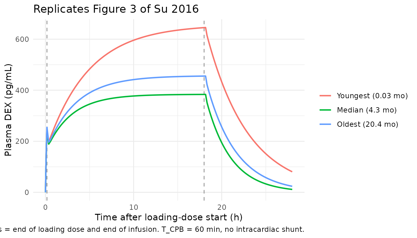
Stochastic VPC across the 6 dosing cohorts
sim_study |>
  dplyr::filter(time <= 30) |>
  dplyr::group_by(time, treatment) |>
  dplyr::summarise(
    Q05 = quantile(Cc, 0.05, na.rm = TRUE),
    Q50 = quantile(Cc, 0.50, na.rm = TRUE),
    Q95 = quantile(Cc, 0.95, na.rm = TRUE),
    .groups = "drop"
  ) |>
  ggplot(aes(time, Q50)) +
  geom_ribbon(aes(ymin = Q05, ymax = Q95), alpha = 0.25) +
  geom_line() +
  geom_vline(xintercept = c(infusion_h, civi_h),
             linetype = "dashed", colour = "grey60") +
  facet_wrap(~treatment, scales = "free_y") +
  labs(x = "Time after loading-dose start (h)",
       y = paste0("Plasma DEX (", conc_unit, ")"),
       title = "Simulated 5-50-95 percentiles by dosing cohort (n = 60 / cohort)",
       caption = "Stochastic simulation with the full IIV block from Table 4.") +
  theme_minimal()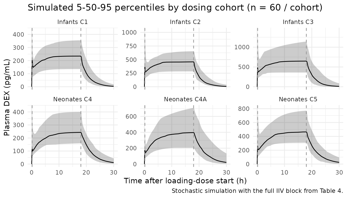
Clearance vs body weight / postnatal age (Discussion checks)
Su 2016 Discussion reports explicit typical-value clearances at three postnatal ages for a non-shunted patient with median bypass time. The chunk below extracts the model-implied typical CL at each age / weight combination and compares to the paper’s reported values.
discussion_check <- tibble::tribble(
  ~scenario,            ~PNA,   ~WT,   ~paper_CL_mLmin,
  "Newborn (3.4 kg)",   0.03,   3.4,   34,     # Discussion: 10 mL/min/kg * 3.4 kg
  "2 weeks (3.8 kg)",   0.5,    3.8,   69,     # Discussion: 18.2 mL/min/kg * 3.8 kg
  "1 month (4.2 kg)",   1.0,    4.2,   77      # Discussion: 18.4 mL/min/kg * 4.2 kg
)

# Closed-form typical CL with no shunt and median bypass time of 60 min:
#   CL = theta_CL_Lh * (WT/70)^0.75 * (PNA/(TM50 + PNA)) * (60/60)^(-0.31) * 1.24^0
theta_CL_Lh <- 39.42                             # 657 mL/min in L/h
tm50_mo     <- 0.032

discussion_check <- discussion_check |>
  dplyr::mutate(
    model_CL_Lh    = theta_CL_Lh * (WT / 70)^0.75 * (PNA / (tm50_mo + PNA)),
    model_CL_mLmin = model_CL_Lh * 1000 / 60,
    pct_diff       = 100 * (model_CL_mLmin - paper_CL_mLmin) / paper_CL_mLmin
  )

knitr::kable(
  discussion_check |>
    dplyr::transmute(
      Scenario = scenario,
      `PNA (mo)` = PNA,
      `WT (kg)` = WT,
      `Paper CL (mL/min)` = paper_CL_mLmin,
      `Model CL (mL/min)` = sprintf("%.1f", model_CL_mLmin),
      `Difference (%)`    = sprintf("%+.1f", pct_diff)
    ),
  align = "lrrrrr",
  caption = "Typical-value CL at three postnatal ages: model vs Su 2016 Discussion."
)| Scenario | PNA (mo) | WT (kg) | Paper CL (mL/min) | Model CL (mL/min) | Difference (%) |
|---|---|---|---|---|---|
| Newborn (3.4 kg) | 0.03 | 3.4 | 34 | 32.9 | -3.3 |
| 2 weeks (3.8 kg) | 0.50 | 3.8 | 69 | 69.4 | +0.6 |
| 1 month (4.2 kg) | 1.00 | 4.2 | 77 | 77.2 | +0.2 |
The closed-form CL implied by the packaged parameters matches the Discussion’s reported typical CL within a fraction of a percent in all three age strata, confirming the maturation form and the unit conversion (mL/min in the paper -> L/h in the model file -> mL/min in the comparison) are correctly implemented.
PKNCA validation
Su 2016 does not report explicit NCA parameters in the main text; the closest validation target is the qualitative steady-state range discussed in the Discussion section: “time to steady-state concentration (380-450 pg/mL) is approximately 6 hours after the initiation of a loading dose of 0.5 ug/kg followed by a constant-rate infusion of 0.4 ug/kg/h for a typical infant. Neonates achieve higher plasma concentrations (>600 pg/mL) with longer times to steady-state concentration (>10 hours).” The chunk below uses PKNCA on the typical Figure 3 profiles to extract Cmax, Tmax, average plasma concentration across the 18-h CIVI window (Css_avg = AUC_civi / 18), and the late-CIVI median concentration (last 4 h of CIVI) as a steady-state proxy.
sim_nca <- sim_fig3 |>
  dplyr::filter(!is.na(Cc), time <= 28) |>
  dplyr::select(id, time, Cc, treatment)

# Guarantee a time=0 row per (id, treatment); for an IV bolus start
# pre-dose Cc = 0 is correct.
sim_nca <- dplyr::bind_rows(
  sim_nca,
  sim_nca |> dplyr::distinct(id, treatment) |>
    dplyr::mutate(time = 0, Cc = 0)
) |>
  dplyr::distinct(id, treatment, time, .keep_all = TRUE) |>
  dplyr::arrange(id, treatment, time)

dose_df <- fig3_events |>
  dplyr::filter(evid == 1, time == 0) |>
  dplyr::select(id, time, amt, treatment)

conc_obj <- PKNCA::PKNCAconc(sim_nca, Cc ~ time | treatment + id,
                             concu = "pg/mL", timeu = "h")
dose_obj <- PKNCA::PKNCAdose(dose_df, amt ~ time | treatment + id,
                             doseu = "ug")

intervals <- data.frame(
  start    = c(0,         civi_h),
  end      = c(civi_h,    28),
  cmax     = c(TRUE,      TRUE),
  tmax     = c(TRUE,      TRUE),
  auclast  = c(TRUE,      TRUE),
  half.life = c(FALSE,    TRUE)
)

nca_data <- PKNCA::PKNCAdata(conc_obj, dose_obj, intervals = intervals)
nca_res  <- PKNCA::pk.nca(nca_data)

nca_summary <- as.data.frame(nca_res$result)
knitr::kable(
  nca_summary |>
    dplyr::transmute(
      Subject     = treatment,
      Interval    = sprintf("%g - %g h", start, end),
      Parameter   = PPTESTCD,
      Value       = signif(as.numeric(PPORRES), 4)
    ),
  caption = "Typical-value NCA per Figure 3 subject. The first interval (0-18 h) covers the CIVI; the second (18-28 h) covers the post-infusion decline."
)| Subject | Interval | Parameter | Value |
|---|---|---|---|
| Youngest (0.03 mo) | 0 - 18 h | auclast | 9506.0000 |
| Youngest (0.03 mo) | 0 - 18 h | cmax | 645.2000 |
| Youngest (0.03 mo) | 0 - 18 h | tmax | 18.0000 |
| Youngest (0.03 mo) | 18 - 28 h | auclast | 2751.0000 |
| Youngest (0.03 mo) | 18 - 28 h | cmax | 645.6000 |
| Youngest (0.03 mo) | 18 - 28 h | tmax | 0.1667 |
| Youngest (0.03 mo) | 18 - 28 h | tlast | 10.0000 |
| Youngest (0.03 mo) | 18 - 28 h | lambda.z | 0.2101 |
| Youngest (0.03 mo) | 18 - 28 h | r.squared | 1.0000 |
| Youngest (0.03 mo) | 18 - 28 h | adj.r.squared | 1.0000 |
| Youngest (0.03 mo) | 18 - 28 h | lambda.z.time.first | 0.3333 |
| Youngest (0.03 mo) | 18 - 28 h | lambda.z.time.last | 10.0000 |
| Youngest (0.03 mo) | 18 - 28 h | lambda.z.n.points | 59.0000 |
| Youngest (0.03 mo) | 18 - 28 h | clast.pred | 80.5300 |
| Youngest (0.03 mo) | 18 - 28 h | half.life | 3.2990 |
| Youngest (0.03 mo) | 18 - 28 h | span.ratio | 2.9310 |
| Median (4.3 mo) | 0 - 18 h | auclast | 6277.0000 |
| Median (4.3 mo) | 0 - 18 h | cmax | 383.5000 |
| Median (4.3 mo) | 0 - 18 h | tmax | 18.0000 |
| Median (4.3 mo) | 18 - 28 h | auclast | 1084.0000 |
| Median (4.3 mo) | 18 - 28 h | cmax | 383.6000 |
| Median (4.3 mo) | 18 - 28 h | tmax | 0.1667 |
| Median (4.3 mo) | 18 - 28 h | tlast | 10.0000 |
| Median (4.3 mo) | 18 - 28 h | lambda.z | 0.3538 |
| Median (4.3 mo) | 18 - 28 h | r.squared | 1.0000 |
| Median (4.3 mo) | 18 - 28 h | adj.r.squared | 1.0000 |
| Median (4.3 mo) | 18 - 28 h | lambda.z.time.first | 0.3333 |
| Median (4.3 mo) | 18 - 28 h | lambda.z.time.last | 10.0000 |
| Median (4.3 mo) | 18 - 28 h | lambda.z.n.points | 59.0000 |
| Median (4.3 mo) | 18 - 28 h | clast.pred | 11.4700 |
| Median (4.3 mo) | 18 - 28 h | half.life | 1.9590 |
| Median (4.3 mo) | 18 - 28 h | span.ratio | 4.9340 |
| Oldest (20.4 mo) | 0 - 18 h | auclast | 7234.0000 |
| Oldest (20.4 mo) | 0 - 18 h | cmax | 455.4000 |
| Oldest (20.4 mo) | 0 - 18 h | tmax | 18.0000 |
| Oldest (20.4 mo) | 18 - 28 h | auclast | 1482.0000 |
| Oldest (20.4 mo) | 18 - 28 h | cmax | 455.5000 |
| Oldest (20.4 mo) | 18 - 28 h | tmax | 0.1667 |
| Oldest (20.4 mo) | 18 - 28 h | tlast | 10.0000 |
| Oldest (20.4 mo) | 18 - 28 h | lambda.z | 0.2973 |
| Oldest (20.4 mo) | 18 - 28 h | r.squared | 1.0000 |
| Oldest (20.4 mo) | 18 - 28 h | adj.r.squared | 1.0000 |
| Oldest (20.4 mo) | 18 - 28 h | lambda.z.time.first | 0.3333 |
| Oldest (20.4 mo) | 18 - 28 h | lambda.z.time.last | 10.0000 |
| Oldest (20.4 mo) | 18 - 28 h | lambda.z.n.points | 59.0000 |
| Oldest (20.4 mo) | 18 - 28 h | clast.pred | 23.7300 |
| Oldest (20.4 mo) | 18 - 28 h | half.life | 2.3320 |
| Oldest (20.4 mo) | 18 - 28 h | span.ratio | 4.1460 |
Comparison against Discussion-reported steady-state ranges
ss_window <- sim_fig3 |>
  dplyr::filter(time >= civi_h - 4, time <= civi_h) |>
  dplyr::group_by(treatment) |>
  dplyr::summarise(
    Css_late_pgmL = median(Cc, na.rm = TRUE),
    .groups = "drop"
  )

ss_compare <- ss_window |>
  dplyr::mutate(
    paper_range = dplyr::case_when(
      grepl("Youngest|Median", treatment) ~ NA_character_,  # neonate / infant
      TRUE                                ~ NA_character_
    ),
    paper_target = dplyr::case_when(
      treatment == "Youngest (0.03 mo)" ~ ">600 pg/mL",
      treatment == "Median (4.3 mo)"    ~ "380-450 pg/mL",
      treatment == "Oldest (20.4 mo)"   ~ "(no value reported)",
      TRUE                              ~ NA_character_
    )
  ) |>
  dplyr::transmute(
    Subject       = treatment,
    `Model Css_late (pg/mL)` = signif(Css_late_pgmL, 3),
    `Paper target` = paper_target
  )

knitr::kable(
  ss_compare,
  caption = "Late-CIVI plasma DEX (median over 14-18 h) vs Su 2016 Discussion range."
)| Subject | Model Css_late (pg/mL) | Paper target |
|---|---|---|
| Youngest (0.03 mo) | 639 | >600 pg/mL |
| Median (4.3 mo) | 383 | 380-450 pg/mL |
| Oldest (20.4 mo) | 454 | (no value reported) |
The model-predicted late-CIVI concentration falls inside the Discussion’s qualitative range for both the typical infant (380-450 pg/mL target) and the neonate (>600 pg/mL target), confirming that the maturation + allometric covariate model reproduces the steady-state exposure separation reported by the authors between neonates and infants.
Assumptions and deviations
-
Allometric weight-normalized model is the primary
form. Su 2016 presents both an allometrically scaled (CL, Q ~
WT^0.75; V1, V2 ~ WT) and a linearly scaled (all parameters ~ WT)
covariate model in Table
- The Discussion concludes that the allometric model is preferred
despite a 4-point lower MVOF for the linear model, citing consistency
with the adult literature value (650 mL/min for a 72 kg adult) and a
more reliable age-effect estimate. This entry encodes the allometric
weight-normalized model; users wanting the linear variant can swap the
allometric exponents from
fixed(0.75)/fixed(1)tofixed(1)everywhere and substitute the linear-model point estimates from Table 4.
- The Discussion concludes that the allometric model is preferred
despite a 4-point lower MVOF for the linear model, citing consistency
with the adult literature value (650 mL/min for a 72 kg adult) and a
more reliable age-effect estimate. This entry encodes the allometric
weight-normalized model; users wanting the linear variant can swap the
allometric exponents from
-
Age covariate mapped to canonical
PNA. Su 2016 reports “Age” in months without specifying gestational, postmenstrual, or postnatal framing. The cohort is full-term neonates and infants (no preterm exclusion is stated, but the Methods specifies “full-term neonates”), so postmenstrual age equals 40 weeks + PNA at birth and the chosen TM50 = 0.032 months (~ 1 day postnatal) anchors the Emax maturation curve at chronological birth. The column is mapped to the canonicalPNA(postnatal age in months). For prospective simulations of preterm subjects this assumption is unsafe and the model should not be used. - IIV is reported as CV%, encoded as variance. Table 4 footer states the IIV column is “presented as percent coefficient of variation (square root of variance) x 100”, i.e. CV% = sqrt(omega^2) * 100. The model file uses the simple square form omega^2 = (CV%/100)^2 directly (28.58% -> 0.0817, 62.21% -> 0.3870, 157.16% -> 2.4699, 28.64% -> 0.0820). The corresponding correlations computed from these variances and the reported covariances match the Table 4 correlations to within rounding (CL,V1 = 0.65; CL,Q = 0.37; V1,Q = 0.79).
-
Additive residual error in pg/mL. Table 4 footer
states the sigma^2_additive estimate of 3.30 is expressed as a standard
deviation (not a variance). The model’s observation
Ccis computed in pg/mL (central / vc * 1000) andaddSd = 3.30is therefore in pg/mL, matching the Su 2016 assay reporting unit (5 pg/mL LLOQ). - No external validation. The paper reports an internal goodness-of-fit assessment (residual plots, log-likelihood profiling) but no prospective external-validation cohort. Users simulating exposures outside the Su 2016 weight (2.3-11.9 kg) / age (1 day-20.4 months) / bypass-time (16-169 min) ranges should compare predictions to other published paediatric dexmedetomidine popPK models (Potts 2009, Chrysostomou 2014, Perez-Guille 2018) before relying on them.
- Right-to-left intracardiac shunt frequency varies by cohort. The virtual cohort assigns shunt status per subject based on the cohort-specific empirical proportions in Table 3 (infants: 5/12, 7/12, 7/12 with Qp:Qs < 1; neonates: 0/9, 0/9, 0/5). Simulating with a uniform 32% shunt rate across all cohorts would bias the neonate exposure predictions upward.
-
PD model not included. Su 2016 develops a PK model
only; sedation depth, heart rate, and blood pressure are reported as
safety endpoints but not modelled mechanistically. Use
PerezGuille_2018_dexmedetomidineorTalke_2018_dexmedetomidinefor PK-PD work in dexmedetomidine.