Tramadol and O-desmethyltramadol (Lee 2019)
Source:vignettes/articles/Lee_2019_tramadol.Rmd
Lee_2019_tramadol.RmdModel and source
#> ℹ parameter labels from comments will be replaced by 'label()'- Citation: Lee J, Yoo HD, Bae JW, Lee S, Shin KH. Population pharmacokinetic analysis of tramadol and O-desmethyltramadol with genetic polymorphism of CYP2D6. Drug Des Devel Ther. 2019;13:1751-1761. doi:10.2147/DDDT.S199574.
- Description: Joint parent-and-metabolite population PK model for sustained-release oral tramadol and its active CYP2D6-derived metabolite O-desmethyltramadol (M1) in healthy Korean male volunteers (Lee 2019). One-compartment disposition for tramadol with two PARALLEL absorption inputs that together deliver one dose: a fraction Fr enters a depot and is absorbed first-order at ka, and the complementary fraction 1 - Fr enters the central compartment as a lagged zero-order input of duration D2, which is how the authors captured the bimodal absorption phase of the extended-release formulation. Tramadol leaves the central compartment by two parallel first-order routes – a non-M1 elimination clearance CL/F and a formation clearance CLPM/F into a one-compartment M1 pool that is itself eliminated by CLM/F. The CYP2D610/10 genotype lowers both the tramadol elimination clearance (by 35.1 percent) and the M1 formation clearance (by 52.8 percent) relative to the wild-type reference group.
- Article: https://doi.org/10.2147/DDDT.S199574
Lee et al. fitted tramadol and its active CYP2D6-derived metabolite O-desmethyltramadol (M1) simultaneously in 22 healthy Korean male volunteers who each took 100 mg of a sustained-release tramadol tablet every 12 h for five doses. The paper is open access; there is no supplement and no NONMEM control stream, so every value below is traced to the main text, Table 2 or Figure 2.
An erratum search (PubMed, the Dove Press article landing page and its corrections feed, and a Google Scholar title search) returned no correction notice for this article.
Population
22 of the 23 enrolled volunteers entered the final model: one subject carrying CYP2D6*5/*5 was excluded before modelling (Lee 2019 Methods, “Population PK model development”). All were Korean men aged 20-40 years (mean 24.8, SD 4.8), weighing 57-90 kg (mean 71.6, SD 8.9), 163-187 cm tall, with BMI 18.1-26.9 kg/m2 (Table 1). The genotype split among the 22 modelled subjects was 14 CYP2D6*wt/*wt and 8 CYP2D6*10/*10; no heterozygous *10 carrier was enrolled, and subjects with a *5 allele or a duplicated CYP2D6 gene were excluded at screening.
Blood was drawn at 0, 0.5, 1, 1.5, 2, 2.5, 3, 4, 6, 8, 10, 12, 24, 48 and 72 h after the fifth dose, yielding 328 tramadol and 323 M1 concentrations. The assay was LC-MS/MS over 1-1000 ng/mL (tramadol) and 1-500 ng/mL (M1). Estimation was by NONMEM 7.3 ADVAN6 with first-order conditional estimation and eta-epsilon interaction.
The same information is available programmatically via
readModelDb("Lee_2019_tramadol")()$population.
Model structure
Figure 2 of the paper draws the model explicitly, and the packaged file reproduces it one arrow at a time:
-
Two parallel absorption inputs for one dose. A
fraction
Fr= 0.88 entersdepotand is absorbed first order atka= 0.095 1/h (absorption half-life 7.3 h, the sustained-release arm). The complementary 0.12 enterscentraldirectly as a zero-order input of durationD2= 1.93 h that starts after a lagALAG2= 1.63 h. Lee 2019 Results: “We applied combined first- and zero-order absorption to catch the bimodal absorption phase of the extended release formulation of tramadol.” -
Two parallel exits from the tramadol compartment.
k20= CL/F / Vp/F is the non-M1 elimination route andk23= CLPM/F / Vp/F is the M1 formation route, so the total apparent tramadol clearance is CL/F + CLPM/F. -
One metabolite compartment eliminated by
k30= CLM/F / Vm/F.
| Item | Encoding |
|---|---|
| ODE states | depot, central, central_m1 |
| Observations | Cc, Cc_m1 |
| Analytic solution used? | no (explicit ODEs) |
How the two absorption inputs are dosed
Each 100 mg administration is written as two event records at
the same time carrying the same amt: one bolus
into depot and one zero-order input into
central. The f(depot) <- ffo /
f(central) <- 1 - ffo lines in the model apportion the
dose between them, so the total delivered is one dose, not two.
The zero-order record is given an explicit numeric
rate, amt * (1 - Fr) / D2, rather
than the usual rate = -2 request for the modelled duration.
rate = -2 currently fails in rxode2 5.1.8 for this
particular combination – a two-endpoint model with both
dur() and alag() on the infused compartment,
plus a second dose record at the same time – with
Duration is zero/negative. The failure disappears if either
endpoint is removed or the alag() is dropped, so it is a
solver interaction, not a model defect. See “Assumptions and
deviations”.
The substitution is checked below rather than asserted in prose: on
the zero-order arm alone (which rate = -2 does solve), the
two encodings must give the same profile to solver precision.
# Fraction of the dose taking the first-order route; no IIV was reported on Fr,
# so this is a single number for every subject.
FFO <- plogis(as.numeric(ui$theta[["logitffo"]]))
stopifnot(abs(FFO - 0.88) < 1e-8)

# knitr::kable() emits markdown and pandoc reads a bare '*' as an emphasis
# marker, so "CYP2D6*10/*10" would render as "CYP2D610/10". Escape asterisks
# for DISPLAY only; the grouping labels themselves keep the published form.
md_esc <- function(x) gsub("*", "\\*", x, fixed = TRUE)

# Build an event table. `subj` must carry id, CYP2D6_STAR10_HOM and d1 (the
# subject's zero-order duration, needed to set the infusion rate).
make_events <- function(subj, n_doses, obs_times, tau = 12) {
  dose_times <- (seq_len(n_doses) - 1) * tau
  dose <- subj |>
    tidyr::crossing(time = dose_times) |>
    dplyr::mutate(amt = 100, evid = 1L, dvid = NA_integer_)
  dose <- dplyr::bind_rows(
    dose |> dplyr::mutate(cmt = "depot", rate = 0),
    dose |> dplyr::mutate(cmt = "central", rate = 100 * (1 - FFO) / d1)
  )
  obs <- subj |>
    tidyr::crossing(time = obs_times) |>
    dplyr::mutate(
      amt = NA_real_, evid = 0L, cmt = "central", rate = 0, dvid = 1L
    )
  dplyr::bind_rows(dose, obs) |>
    dplyr::select(-d1) |>
    dplyr::arrange(id, time, dplyr::desc(evid))
}
# Zero-order arm ONLY (no depot record), so rate = -2 solves. The numeric-rate
# substitution used everywhere else must reproduce it exactly.
d1_ref <- exp(as.numeric(ui$theta[["ld1"]]))
grid_eq <- seq(0, 48, by = 0.1)
ev_eq <- function(rate_value) {
  ev <- dplyr::bind_rows(
    data.frame(
      id = 1L, time = 0, amt = 100, evid = 1L, cmt = "central",
      rate = rate_value, dvid = NA_integer_
    ),
    data.frame(
      id = 1L, time = grid_eq, amt = NA_real_, evid = 0L, cmt = "central",
      rate = 0, dvid = 1L
    )
  )
  ev$CYP2D6_STAR10_HOM <- 0
  ev
}
mod_typ <- ui |> rxode2::zeroRe()
eq_modelled <- rxode2::rxSolve(mod_typ, ev_eq(-2), useLinCmt = FALSE) |>
  as.data.frame()
#> ℹ omega/sigma items treated as zero: 'etalcl', 'etalvc', 'etalcl_form_m1', 'etald1'
eq_numeric <- rxode2::rxSolve(
  mod_typ, ev_eq(100 * (1 - FFO) / d1_ref),
  useLinCmt = FALSE
) |>
  as.data.frame()
#> ℹ omega/sigma items treated as zero: 'etalcl', 'etalvc', 'etalcl_form_m1', 'etald1'
# Relative to the peak, because the residual is ODE-solver tolerance (rxode2
# defaults to rtol 1e-6), not a difference between the two encodings. A
# genuinely different infusion duration moves the profile by percent, so 1e-5
# separates "same solution" from "different model" by three orders of magnitude.
rate_agreement <- max(abs(eq_modelled$Cc - eq_numeric$Cc)) / max(eq_modelled$Cc)
stopifnot(nrow(eq_modelled) == length(grid_eq), rate_agreement < 1e-5)
The two encodings agree to 4.9^{-10} of the peak concentration, i.e. to the solver’s own tolerance.
Source trace
Every ini() entry in
inst/modeldb/specificDrugs/Lee_2019_tramadol.R carries an
in-file comment naming its source location; they are collected here for
review.
| Equation / parameter | Value | Source location |
|---|---|---|
lcl (CL/F) |
16.9 L/h | Table 2, row “CL/F (L/hr)” |
lvc (Vp/F) |
59.9 L | Table 2, row “Vp/F (L)” |
lka (ka) |
0.095 1/h | Table 2, row “ka (hr-1)” |
ld1 (D2) |
1.93 h | Table 2, row “D2 (hr)” |
ltlag (ALAG2) |
1.63 h | Table 2, row “ALAG2 (hr)” |
logitffo (Fr) |
0.88 | Table 2, row “Fr” |
lcl_form_m1 (CLPM/F) |
4.11 L/h | Table 2, row “CLPM/F (L/hr)” |
lcl_m1 (CLM/F) |
15.8 L/h | Table 2, row “CLM/F (L/hr)” |
lvc_m1 (Vm/F) |
8.63 L | Table 2, row “Vm/F (L)” |
e_cyp2d6_star10_hom_cl |
0.351 | Table 2, row “CL/F, CYP2D6*10/*10”; Results equation CL/F = 16.9 (1 - 0.351 G) |
e_cyp2d6_star10_hom_cl_form_m1 |
0.528 | Table 2, row “CLPM/F, CYP2D6*10/*10”; Results equation CLPM/F = 4.11 (1 - 0.528 G) |
etalcl |
0.059 | Table 2, row “omega^2 CL/F” (a variance) |
etalvc |
0.023 | Table 2, row “omega^2 V/F” (a variance) |
etalcl_form_m1 |
0.017 | Table 2, row “omega^2 CLPM/F” (a variance) |
etald1 |
0.161 | Table 2, row “omega^2 D2” (a variance) |
propSd |
0.13 | Table 2, row “sigma pro,tra”; Results “13%” |
addSd |
2.99 ng/mL | Table 2, row “sigma add,tra”; Results “2.99 ng/mL” |
propSd_m1 |
0.109 | Table 2, row “sigma pro,ODMT”; Results “10.9%” |
addSd_m1 |
1.06 ng/mL | Table 2, row “sigma add,ODMT”; Results “1.06 ng/mL” |
| Parallel first- plus zero-order input, lagged zero-order arm | n/a | Figure 2 scheme (ka/F1 into Depot,
D2/1-F1 into Tramadol); Results
“Pharmacokinetic analysis” |
Two parallel exits k20 (CL) and k23 (CLPM)
from Tramadol |
n/a | Figure 2 scheme |
One-compartment M1 with first-order k30 (CLM) |
n/a | Figure 2 scheme; Results “Pharmacokinetic analysis” |
| Exponential IIV, combined proportional-plus-additive RUV | n/a | Methods “Population PK model development”, unnumbered equations |
Covariate form theta_n1 * (1 - theta_n2 * G)
|
n/a | Methods “Covariates selection”, unnumbered equation |
Typical-value verification of the covariate model
The paper states both covariate-adjusted clearances in words in the Discussion, which makes them a direct, deterministic check on the encoding.
typ_subj <- tibble::tibble(
  id = 1:2,
  genotype = c("CYP2D6*wt/*wt", "CYP2D6*10/*10"),
  CYP2D6_STAR10_HOM = c(0, 1),
  d1 = exp(as.numeric(ui$theta[["ld1"]]))
)

# A grid that is fine through absorption and the two zero-order kinks, and long
# enough for the tramadol terminal phase (absorption-rate limited, t1/2 7.3 h).
grid_sd <- sort(unique(c(
  seq(0, 24, by = 0.02), seq(24, 96, by = 0.25), seq(96, 480, by = 1)
)))

sim_typ <- rxode2::rxSolve(
  mod_typ,
  make_events(typ_subj, n_doses = 1L, obs_times = grid_sd),
  keep = "genotype",
  # rxode2's automatic ODE -> linCmt() conversion corrupts the dvid mapping for
  # multi-output models.
  useLinCmt = FALSE
) |>
  as.data.frame()
#> ℹ omega/sigma items treated as zero: 'etalcl', 'etalvc', 'etalcl_form_m1', 'etald1'
#> Warning: multi-subject simulation without without 'omega'

cl_tab <- sim_typ |>
  dplyr::group_by(genotype) |>
  dplyr::summarise(
    `CL/F (L/h)` = dplyr::first(cl),
    `CLPM/F (L/h)` = dplyr::first(cl_form_m1),
    `CLM/F (L/h)` = dplyr::first(cl_m1),
    `Total tramadol CL/F (L/h)` = dplyr::first(cl) + dplyr::first(cl_form_m1),
    .groups = "drop"
  )

knitr::kable(
  cl_tab |>
    dplyr::mutate(genotype = md_esc(genotype)) |>
    dplyr::rename("Genotype" = genotype),
  digits = 3,
  caption = "Typical apparent clearances by CYP2D6 star-10 genotype."
)| Genotype | CL/F (L/h) | CLPM/F (L/h) | CLM/F (L/h) | Total tramadol CL/F (L/h) |
|---|---|---|---|---|
| CYP2D6*10/*10 | 10.968 | 1.94 | 15.8 | 12.908 |
| CYP2D6*wt/*wt | 16.900 | 4.11 | 15.8 | 21.010 |
# Lee 2019 Discussion: "CL/F was estimated as 16.9 L/hr for wild type, and
# 11.0 L/hr for the CYP2D6*10/*10 group, while CLPM/F was estimated as 4.11
# L/hr and 1.94 L/hr for wild type and CYP2D6*10/*10 group, respectively."
# These are exact algebraic consequences of the ini() values, so the tolerance
# only has to absorb the paper's own rounding to 3 significant figures.
cl_wt <- cl_tab$`CL/F (L/h)`[cl_tab$genotype == "CYP2D6*wt/*wt"]
cl_hom <- cl_tab$`CL/F (L/h)`[cl_tab$genotype == "CYP2D6*10/*10"]
clpm_wt <- cl_tab$`CLPM/F (L/h)`[cl_tab$genotype == "CYP2D6*wt/*wt"]
clpm_hom <- cl_tab$`CLPM/F (L/h)`[cl_tab$genotype == "CYP2D6*10/*10"]
stopifnot(
  length(cl_wt) == 1L, length(cl_hom) == 1L,
  abs(cl_wt - 16.9) < 1e-8,
  abs(cl_hom - 11.0) < 0.05,
  abs(clpm_wt - 4.11) < 1e-8,
  abs(clpm_hom - 1.94) < 0.005
)
The dose split and the zero-order duration are encoded as published
Two structural identities pin down the absorption model and the two parallel exits. Both are exact for this linear model, so they are asserted tightly; a mis-transcribed clearance, volume, dose split or unit moves them by percent, not parts per million.
# Trapezoidal AUC on the (deterministic) typical-value profile.
trap_auc <- function(time, conc) {
  sum(diff(time) * (utils::head(conc, -1) + utils::tail(conc, -1)) / 2)
}

gates <- sim_typ |>
  dplyr::group_by(genotype) |>
  dplyr::summarise(
    auc = trap_auc(time, Cc),
    auc_m1 = trap_auc(time, Cc_m1),
    cl_tot = dplyr::first(cl) + dplyr::first(cl_form_m1),
    cl_form = dplyr::first(cl_form_m1),
    cl_m1 = dplyr::first(cl_m1),
    ctail = dplyr::last(Cc),
    .groups = "drop"
  ) |>
  dplyr::mutate(
    # Whole dose recovered: (CL/F + CLPM/F) * AUCinf = Dose. 100 mg = 1e5 ng*L/mL.
    dose_recovery = cl_tot * auc / 1e5,
    # Formation flux recovered: CLM/F * AUCinf_M1 = CLPM/F * AUCinf_tramadol.
    m1_recovery = (cl_m1 * auc_m1) / (cl_form * auc)
  )

knitr::kable(
  gates |>
    dplyr::select(genotype, auc, auc_m1, dose_recovery, m1_recovery) |>
    dplyr::mutate(genotype = md_esc(genotype)) |>
    dplyr::rename(
      "Genotype" = genotype,
      "AUCinf tramadol (ng*h/mL)" = auc,
      "AUCinf M1 (ng*h/mL)" = auc_m1,
      "(CL+CLPM) * AUC / Dose" = dose_recovery,
      "CLM * AUC_M1 / (CLPM * AUC)" = m1_recovery
    ),
  digits = c(0, 1, 1, 6, 6),
  caption = "Closed-form mass-balance gates on the typical-value profile."
)| Genotype | AUCinf tramadol (ng*h/mL) | AUCinf M1 (ng*h/mL) | (CL+CLPM) * AUC / Dose | CLM * AUC_M1 / (CLPM * AUC) |
|---|---|---|---|---|
| CYP2D6*10/*10 | 7747.2 | 951.2 | 1.000007 | 1 |
| CYP2D6*wt/*wt | 4759.7 | 1238.1 | 1.000006 | 1 |
stopifnot(
  # The solve is deterministic (no random effects), so the only error here is
  # trapezoidal. Realised 3e-6 on this grid; 1e-3 leaves three orders of
  # magnitude of headroom and still breaks on any transcription error.
  all(abs(gates$dose_recovery - 1) < 1e-3),
  all(abs(gates$m1_recovery - 1) < 1e-3),
  # The profile has actually decayed, so AUCinf is not truncated.
  all(gates$ctail / (gates$auc / 480) < 1e-6)
)

# The zero-order arm really is zero-order, of duration D2, starting at ALAG2:
# dCc/dt must step UP by exactly the zero-order input rate at ALAG2 and step
# back DOWN by the same amount at ALAG2 + D2.
tlag_i <- exp(as.numeric(ui$theta[["ltlag"]]))
d1_i <- exp(as.numeric(ui$theta[["ld1"]]))
vc_i <- exp(as.numeric(ui$theta[["lvc"]]))
zo_rate_conc <- 1000 * 100 * (1 - FFO) / d1_i / vc_i

slope <- sim_typ |>
  dplyr::filter(genotype == "CYP2D6*wt/*wt", time <= 8) |>
  dplyr::mutate(dC = c(NA, diff(Cc) / diff(time)))
slope_at <- function(t) slope$dC[which.min(abs(slope$time - t))]

jump_up <- slope_at(tlag_i + 0.1) - slope_at(tlag_i - 0.1)
jump_down <- slope_at(tlag_i + d1_i - 0.1) - slope_at(tlag_i + d1_i + 0.1)

knitr::kable(
  tibble::tibble(
    "Zero-order kink" = c("start (ALAG2)", "end (ALAG2 + D2)"),
    "Time (h)" = c(tlag_i, tlag_i + d1_i),
    "Step in dCc/dt (ng/mL/h)" = c(jump_up, jump_down),
    "Expected (ng/mL/h)" = zo_rate_conc
  ),
  digits = 2,
  caption = "The zero-order arm delivers (1 - Fr) x Dose over D2, starting at ALAG2."
)| Zero-order kink | Time (h) | Step in dCc/dt (ng/mL/h) | Expected (ng/mL/h) |
|---|---|---|---|
| start (ALAG2) | 1.63 | 94.14 | 103.8 |
| end (ALAG2 + D2) | 3.56 | 107.45 | 103.8 |
Virtual cohort
The observed data are not public, so the figures below use a virtual cohort of 200 subjects per genotype arm drawn from the published OMEGA.
The between-subject random effects are drawn in R
with stats::rnorm and passed to rxSolve() as
per-subject typical values on a model whose random effects have been
zeroed. Two reasons: the subject’s zero-order duration D2
has to be known before the event table can be written (it sets the
infusion rate, see above), and drawing in R makes the cohort
reproducible across machines and solver-thread counts, which
rxode2::rxSetSeed() alone cannot guarantee. The published
OMEGA is diagonal, so independent normal draws reproduce it exactly.
set.seed(20190601)

n_per_arm <- 200L
omega <- ui$omega
stopifnot(
  # Independent draws below are only equivalent to the published OMEGA because
  # the paper reports no covariances.
  isTRUE(all.equal(omega, diag(diag(omega)), check.attributes = FALSE)),
  identical(
    dimnames(omega)[[1]],
    c("etalcl", "etalvc", "etalcl_form_m1", "etald1")
  )
)

draw_arm <- function(n, genotype, star10_hom, id_offset) {
  tibble::tibble(
    id = id_offset + seq_len(n),
    genotype = genotype,
    CYP2D6_STAR10_HOM = star10_hom,
    etalcl = stats::rnorm(n, 0, sqrt(omega["etalcl", "etalcl"])),
    etalvc = stats::rnorm(n, 0, sqrt(omega["etalvc", "etalvc"])),
    etalcl_form_m1 = stats::rnorm(
      n, 0, sqrt(omega["etalcl_form_m1", "etalcl_form_m1"])
    ),
    etald1 = stats::rnorm(n, 0, sqrt(omega["etald1", "etald1"]))
  )
}

cohort <- dplyr::bind_rows(
  draw_arm(n_per_arm, "CYP2D6*wt/*wt", 0, 0L),
  draw_arm(n_per_arm, "CYP2D6*10/*10", 1, n_per_arm)
) |>
  dplyr::mutate(
    lcl = as.numeric(ui$theta[["lcl"]]) + etalcl,
    lvc = as.numeric(ui$theta[["lvc"]]) + etalvc,
    lcl_form_m1 = as.numeric(ui$theta[["lcl_form_m1"]]) + etalcl_form_m1,
    ld1 = as.numeric(ui$theta[["ld1"]]) + etald1,
    d1 = exp(ld1)
  )

cohort_params <- cohort |>
  dplyr::select(id, lcl, lvc, lcl_form_m1, ld1)

events <- make_events(
  cohort |> dplyr::select(id, genotype, CYP2D6_STAR10_HOM, d1),
  n_doses = 1L,
  obs_times = sort(unique(c(
    seq(0, 24, by = 0.2), seq(24, 96, by = 0.5), seq(96, 360, by = 2)
  )))
)
stopifnot(!anyDuplicated(unique(events[, c("id", "time", "evid", "cmt")])))
Simulation
sim <- rxode2::rxSolve(
  mod_typ,
  events,
  params = cohort_params,
  keep = "genotype",
  useLinCmt = FALSE
) |>
  as.data.frame()
#> ℹ omega/sigma items treated as zero: 'etalcl', 'etalvc', 'etalcl_form_m1', 'etald1'
#> Warning: multi-subject simulation without without 'omega'

# The per-subject typical values really did reach the solver: each subject's
# cl must be exp(lcl_i) times its own genotype factor, and likewise for the
# formation clearance. This is the guard against rxSolve silently recycling
# the population typical value instead of the supplied per-subject row.
e_cl <- as.numeric(ui$theta[["e_cyp2d6_star10_hom_cl"]])
e_clpm <- as.numeric(ui$theta[["e_cyp2d6_star10_hom_cl_form_m1"]])

chk <- sim |>
  dplyr::group_by(id) |>
  dplyr::summarise(
    cl = dplyr::first(cl),
    cl_form_m1 = dplyr::first(cl_form_m1),
    .groups = "drop"
  ) |>
  dplyr::inner_join(
    cohort |> dplyr::select(id, lcl, lcl_form_m1, CYP2D6_STAR10_HOM),
    by = "id"
  ) |>
  dplyr::mutate(
    cl_expected = exp(lcl) * (1 - e_cl * CYP2D6_STAR10_HOM),
    cl_form_expected = exp(lcl_form_m1) * (1 - e_clpm * CYP2D6_STAR10_HOM)
  )
stopifnot(
  nrow(chk) == 2L * n_per_arm,
  # Both arms present, so a dropped covariate column would break this too.
  dplyr::n_distinct(chk$CYP2D6_STAR10_HOM) == 2L,
  max(abs(chk$cl - chk$cl_expected)) < 1e-8,
  max(abs(chk$cl_form_m1 - chk$cl_form_expected)) < 1e-8
)
Simulated concentration-time profiles (replicates Figure 1)
Figure 1 of Lee 2019 shows the observed mean tramadol and M1 profiles for 72 h after the last of five doses, stratified by CYP2D6 genotype, on a log concentration axis. The single-dose cohort here reproduces the same qualitative separation: tramadol exposure is higher and M1 exposure lower in CYP2D6*10/*10 subjects.
sim |>
  dplyr::filter(time <= 72) |>
  dplyr::select(id, genotype, time, Tramadol = Cc, `M1` = Cc_m1) |>
  tidyr::pivot_longer(c(Tramadol, `M1`), names_to = "analyte", values_to = "conc") |>
  dplyr::group_by(analyte, genotype, time) |>
  dplyr::summarise(
    Q05 = quantile(conc, 0.05),
    Q50 = quantile(conc, 0.50),
    Q95 = quantile(conc, 0.95),
    .groups = "drop"
  ) |>
  ggplot(aes(time, Q50, colour = genotype, fill = genotype)) +
  geom_ribbon(aes(ymin = Q05, ymax = Q95), alpha = 0.2, colour = NA) +
  geom_line() +
  facet_wrap(~analyte, scales = "free_y") +
  scale_y_log10() +
  labs(
    x = "Time after a single 100 mg dose (h)",
    y = "Concentration (ng/mL)",
    colour = NULL, fill = NULL,
    title = "Simulated single-dose profiles by CYP2D6*10 genotype",
    caption = "Median and 5th-95th percentile of 200 subjects per arm. Compare Figure 1 of Lee 2019."
  ) +
  theme(legend.position = "bottom")
#> Warning in scale_y_log10(): log-10 transformation introduced infinite values.
#> log-10 transformation introduced infinite values.
#> log-10 transformation introduced infinite values.
#> log-10 transformation introduced infinite values.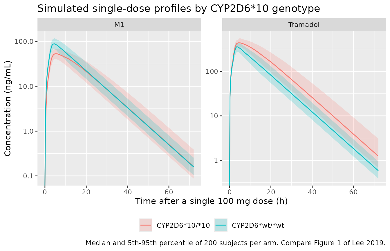
PKNCA validation
NCA is run separately for each analyte, with the genotype arm as the treatment grouping variable.
dose_df <- events |>
  dplyr::filter(evid == 1, cmt == "depot") |>
  dplyr::select(id, time, amt, genotype)
stopifnot(nrow(dose_df) == 2L * n_per_arm)

dose_obj <- PKNCA::PKNCAdose(
  dose_df, amt ~ time | genotype + id,
  doseu = "mg"
)

nca_intervals <- data.frame(
  start = 0, end = Inf,
  cmax = TRUE, tmax = TRUE, aucinf.obs = TRUE,
  half.life = TRUE, clast.obs = TRUE
)

run_nca <- function(conc_df, conc_col) {
  d <- conc_df
  d$Cc <- d[[conc_col]]
  d <- d |>
    dplyr::filter(!is.na(Cc)) |>
    dplyr::select(id, time, genotype, Cc)
  # Guarantee a time-zero anchor; pre-dose concentration is zero for an oral
  # single dose. Without it PKNCA warns once per subject that the AUC range
  # starts before the first measurement.
  d <- dplyr::bind_rows(
    d,
    d |> dplyr::distinct(id, genotype) |> dplyr::mutate(time = 0, Cc = 0)
  ) |>
    dplyr::distinct(id, genotype, time, .keep_all = TRUE) |>
    dplyr::arrange(id, time)
  stopifnot(nrow(d) > 0L, sum(d$time == 0) == 2L * n_per_arm)
  conc_obj <- PKNCA::PKNCAconc(
    d, Cc ~ time | genotype + id,
    concu = "ng/mL", timeu = "h"
  )
  PKNCA::pk.nca(PKNCA::PKNCAdata(conc_obj, dose_obj, intervals = nca_intervals))
}

nca_tramadol <- run_nca(sim, "Cc")
nca_m1 <- run_nca(sim, "Cc_m1")
tidy_nca <- function(res, analyte) {
  as.data.frame(res) |>
    dplyr::filter(PPTESTCD %in% c("cmax", "tmax", "aucinf.obs", "half.life")) |>
    dplyr::group_by(genotype, PPTESTCD) |>
    dplyr::summarise(
      median = stats::median(PPORRES),
      p05 = stats::quantile(PPORRES, 0.05),
      p95 = stats::quantile(PPORRES, 0.95),
      .groups = "drop"
    ) |>
    dplyr::mutate(analyte = analyte)
}

nca_summary <- dplyr::bind_rows(
  tidy_nca(nca_tramadol, "Tramadol"),
  tidy_nca(nca_m1, "O-desmethyltramadol (M1)")
) |>
  dplyr::mutate(
    Parameter = dplyr::recode(
      PPTESTCD,
      cmax = "Cmax (ng/mL)",
      tmax = "Tmax (h)",
      aucinf.obs = "AUC0-inf obs (ng*h/mL)",
      half.life = "t1/2 (h)"
    )
  ) |>
  dplyr::select(analyte, genotype, Parameter, median, p05, p95) |>
  dplyr::arrange(analyte, Parameter, genotype)

nca_summary |>
  dplyr::mutate(genotype = md_esc(genotype)) |>
  dplyr::rename(
    "Analyte" = analyte,
    "Genotype" = genotype,
    "NCA parameter" = Parameter,
    "Median" = median,
    "5th pctile" = p05,
    "95th pctile" = p95
  ) |>
  knitr::kable(
    digits = 2,
    caption = paste(
      "Simulated single-dose NCA (PKNCA) after 100 mg oral tramadol,",
      "200 subjects per genotype arm."
    )
)| Analyte | Genotype | NCA parameter | Median | 5th pctile | 95th pctile |
|---|---|---|---|---|---|
| O-desmethyltramadol (M1) | CYP2D6*10/*10 | AUC0-inf obs (ng*h/mL) | 947.63 | 628.78 | 1391.87 |
| O-desmethyltramadol (M1) | CYP2D6*wt/*wt | AUC0-inf obs (ng*h/mL) | 1222.91 | 868.64 | 1739.19 |
| O-desmethyltramadol (M1) | CYP2D6*10/*10 | Cmax (ng/mL) | 53.90 | 41.01 | 70.23 |
| O-desmethyltramadol (M1) | CYP2D6*wt/*wt | Cmax (ng/mL) | 89.56 | 67.89 | 118.63 |
| O-desmethyltramadol (M1) | CYP2D6*10/*10 | Tmax (h) | 5.30 | 4.20 | 7.20 |
| O-desmethyltramadol (M1) | CYP2D6*wt/*wt | Tmax (h) | 4.40 | 3.60 | 5.60 |
| O-desmethyltramadol (M1) | CYP2D6*10/*10 | t1/2 (h) | 7.36 | 7.33 | 7.38 |
| O-desmethyltramadol (M1) | CYP2D6*wt/*wt | t1/2 (h) | 7.33 | 7.32 | 7.35 |
| Tramadol | CYP2D6*10/*10 | AUC0-inf obs (ng*h/mL) | 7703.88 | 5435.67 | 10898.84 |
| Tramadol | CYP2D6*wt/*wt | AUC0-inf obs (ng*h/mL) | 4708.38 | 3489.01 | 6554.67 |
| Tramadol | CYP2D6*10/*10 | Cmax (ng/mL) | 451.95 | 369.78 | 562.41 |
| Tramadol | CYP2D6*wt/*wt | Cmax (ng/mL) | 373.12 | 296.64 | 460.88 |
| Tramadol | CYP2D6*10/*10 | Tmax (h) | 4.40 | 3.00 | 6.60 |
| Tramadol | CYP2D6*wt/*wt | Tmax (h) | 3.60 | 2.80 | 5.01 |
| Tramadol | CYP2D6*10/*10 | t1/2 (h) | 7.36 | 7.33 | 7.38 |
| Tramadol | CYP2D6*wt/*wt | t1/2 (h) | 7.33 | 7.32 | 7.35 |
All four terminal half-lives come out at about 7.3 h, and they are
the same for the parent and for the metabolite. That is the signature of
flip-flop kinetics: ka = 0.095 1/h gives an absorption
half-life of 7.30 h, while the fastest tramadol elimination half-life is
1.98 h (wild type) and the M1 elimination half-life is only 0.38 h, so
the absorption rate is what the terminal slope measures in every arm and
for both analytes. This is a structural consequence of the published
parameters, not a fitted quantity, so it is asserted directly.
ka_halflife <- log(2) / exp(as.numeric(ui$theta[["lka"]]))
hl <- nca_summary |>
  dplyr::filter(Parameter == "t1/2 (h)") |>
  dplyr::mutate(rel = median / ka_halflife)
stopifnot(
  nrow(hl) == 4L,
  # Realised 1.005-1.009; lambda-z is fitted over a finite window, so it sits
  # slightly above the true asymptote. 3% still breaks if the terminal slope is
  # set by elimination (1.98 h wild type, 0.38 h for M1) instead of absorption.
  all(abs(hl$rel - 1) < 0.03)
)
Lee 2019 reports no NCA table, so there is nothing to place beside
these values with ncaComparisonTable(). The PKNCA output is
instead checked against the model’s own closed-form exposure, which is
the stronger test: for this linear model each subject’s AUC0-inf must
equal Dose / (CL/F + CLPM/F) exactly, and each subject’s M1
AUC0-inf must equal CLPM/F / CLM/F times the tramadol
AUC0-inf.
per_subject <- sim |>
  dplyr::group_by(id, genotype) |>
  dplyr::summarise(
    cl = dplyr::first(cl),
    cl_form_m1 = dplyr::first(cl_form_m1),
    cl_m1 = dplyr::first(cl_m1),
    .groups = "drop"
  ) |>
  dplyr::mutate(
    auc_pred = 1e5 / (cl + cl_form_m1),
    auc_m1_pred = (cl_form_m1 / cl_m1) * auc_pred
  )

auc_obs <- function(res, nm) {
  d <- as.data.frame(res) |>
    dplyr::filter(PPTESTCD == "aucinf.obs") |>
    dplyr::select(id, PPORRES)
  names(d)[2] <- nm
  d
}

auc_cmp <- per_subject |>
  dplyr::inner_join(auc_obs(nca_tramadol, "auc_nca"), by = "id") |>
  dplyr::inner_join(auc_obs(nca_m1, "auc_m1_nca"), by = "id") |>
  dplyr::mutate(
    pct_diff = 100 * (auc_nca - auc_pred) / auc_pred,
    pct_diff_m1 = 100 * (auc_m1_nca - auc_m1_pred) / auc_m1_pred
  )
stopifnot(nrow(auc_cmp) == 2L * n_per_arm)

knitr::kable(
  auc_cmp |>
    dplyr::group_by(genotype) |>
    dplyr::summarise(
      `Tramadol median % diff` = stats::median(pct_diff),
      `Tramadol 90th pctile abs % diff` = stats::quantile(abs(pct_diff), 0.9),
      `M1 median % diff` = stats::median(pct_diff_m1),
      `M1 90th pctile abs % diff` = stats::quantile(abs(pct_diff_m1), 0.9),
      .groups = "drop"
    ) |>
    dplyr::mutate(genotype = md_esc(genotype)) |>
    dplyr::rename("Genotype" = genotype),
  digits = 3,
  caption = "PKNCA AUC0-inf against the model's closed-form AUC, per subject."
)| Genotype | Tramadol median % diff | Tramadol 90th pctile abs % diff | M1 median % diff | M1 90th pctile abs % diff |
|---|---|---|---|---|
| CYP2D6*10/*10 | -0.009 | 0.013 | -0.001 | 0.002 |
| CYP2D6*wt/*wt | -0.015 | 0.022 | -0.002 | 0.003 |
# The remaining difference is trapezoidal error plus PKNCA's extrapolation of
# the terminal tail, both of which depend on where each subject's zero-order
# kinks land on the observation grid. Assert the centre and a robust quantile
# rather than the extreme, and keep the bound loose enough to survive a
# different cohort draw but tight enough to break on a structural error (a
# wrong dose split, volume or clearance moves these by tens of percent).
stopifnot(
  abs(stats::median(auc_cmp$pct_diff)) < 1,
  stats::quantile(abs(auc_cmp$pct_diff), 0.9) < 2,
  abs(stats::median(auc_cmp$pct_diff_m1)) < 1,
  stats::quantile(abs(auc_cmp$pct_diff_m1), 0.9) < 2
)
Steady state: replicating Figure 6
Figure 6 of Lee 2019 simulates tramadol and M1 “during 1 week after twice-daily administration of 100 mg tramadol”, and the Discussion draws the paper’s headline quantitative conclusion from it: “the peak plasma concentration of tramadol for the CYP2D6 genotypes, CYP2D6*10/*10, was approximately 1.5 times higher than that of the wild type (CYP2D6*wt/*wt), at the steady state after multiple tramadol 100 mg twice daily administrations”.
tau <- 12
n_doses_ss <- 15L
last_full <- (n_doses_ss - 2L) * tau # start of the last COMPLETE interval

# Observe past the final dosing interval: rxode2 truncates a lagged infusion at
# the last observation record, which would silently clip the final interval.
grid_ss <- sort(unique(c(
  seq(0, last_full, by = 0.25),
  seq(last_full, last_full + tau, by = 0.02),
  seq(last_full + tau, (n_doses_ss - 1L) * tau + 2 * tau, by = 0.25)
)))

sim_ss <- rxode2::rxSolve(
  mod_typ,
  make_events(typ_subj, n_doses = n_doses_ss, obs_times = grid_ss, tau = tau),
  keep = "genotype",
  useLinCmt = FALSE
) |>
  as.data.frame()
#> ℹ omega/sigma items treated as zero: 'etalcl', 'etalvc', 'etalcl_form_m1', 'etald1'
#> Warning: multi-subject simulation without without 'omega'

sim_ss |>
  dplyr::filter(time <= 168) |>
  dplyr::select(genotype, time, Tramadol = Cc, `M1` = Cc_m1) |>
  tidyr::pivot_longer(c(Tramadol, `M1`), names_to = "analyte", values_to = "conc") |>
  ggplot(aes(time / 24, conc, colour = genotype)) +
  geom_line() +
  facet_wrap(~analyte, scales = "free_y") +
  labs(
    x = "Time (days)", y = "Concentration (ng/mL)", colour = NULL,
    title = "Typical-value profiles, 100 mg twice daily for one week",
    caption = "Replicates Figure 6 of Lee 2019."
  ) +
  theme(legend.position = "bottom")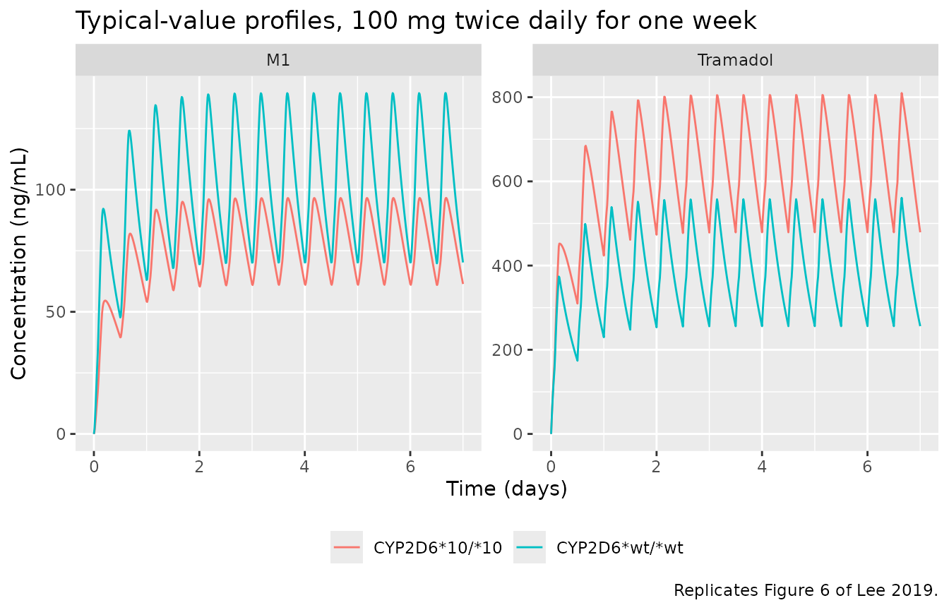
ss_metrics <- sim_ss |>
  dplyr::filter(time >= last_full, time <= last_full + tau) |>
  dplyr::group_by(genotype) |>
  dplyr::summarise(
    cmax = max(Cc),
    tmax = time[which.max(Cc)] - last_full,
    ctrough = dplyr::first(Cc),
    auctau = trap_auc(time, Cc),
    cmax_m1 = max(Cc_m1),
    auctau_m1 = trap_auc(time, Cc_m1),
    cl_tot = dplyr::first(cl) + dplyr::first(cl_form_m1),
    cl_form = dplyr::first(cl_form_m1),
    cl_m1 = dplyr::first(cl_m1),
    .groups = "drop"
  )

knitr::kable(
  ss_metrics |>
    dplyr::select(genotype, cmax, tmax, ctrough, auctau, cmax_m1, auctau_m1) |>
    dplyr::mutate(genotype = md_esc(genotype)) |>
    dplyr::rename(
      "Genotype" = genotype,
      "Tramadol Cmax,ss (ng/mL)" = cmax,
      "Tramadol Tmax,ss (h)" = tmax,
      "Tramadol Ctrough,ss (ng/mL)" = ctrough,
      "Tramadol AUCtau (ng*h/mL)" = auctau,
      "M1 Cmax,ss (ng/mL)" = cmax_m1,
      "M1 AUCtau (ng*h/mL)" = auctau_m1
    ),
  digits = 1,
  caption = "Typical-value steady-state exposure over the last complete 12 h interval."
)| Genotype | Tramadol Cmax,ss (ng/mL) | Tramadol Tmax,ss (h) | Tramadol Ctrough,ss (ng/mL) | Tramadol AUCtau (ng*h/mL) | M1 Cmax,ss (ng/mL) | M1 AUCtau (ng*h/mL) |
|---|---|---|---|---|---|---|
| CYP2D6*10/*10 | 809.9 | 3.6 | 479 | 7747.1 | 96.6 | 951.2 |
| CYP2D6*wt/*wt | 560.9 | 3.6 | 256 | 4759.6 | 139.6 | 1238.1 |
wt <- ss_metrics[ss_metrics$genotype == "CYP2D6*wt/*wt", ]
hom <- ss_metrics[ss_metrics$genotype == "CYP2D6*10/*10", ]
stopifnot(nrow(wt) == 1L, nrow(hom) == 1L)

cmax_ratio <- hom$cmax / wt$cmax
m1_frac_ratio <- (hom$auctau_m1 / hom$auctau) / (wt$auctau_m1 / wt$auctau)

claims <- tibble::tribble(
  ~Claim, ~Source, ~Achieved, ~Pass,
  "Steady-state tramadol Cmax is about 1.5x higher in CYP2D6*10/*10",
  "Discussion", sprintf("%.2fx", cmax_ratio),
  cmax_ratio > 1.25 && cmax_ratio < 1.75,
  "AUCtau at steady state equals single-dose AUCinf (linear superposition)",
  "structural", sprintf("%.6f", hom$auctau / (1e5 / hom$cl_tot)),
  abs(hom$auctau / (1e5 / hom$cl_tot) - 1) < 1e-3,
  "M1-to-tramadol AUC ratio falls by the factor (1 - 0.528) in CYP2D6*10/*10",
  "Table 2 / Results", sprintf("%.5f", m1_frac_ratio),
  abs(m1_frac_ratio - (1 - 0.528)) < 1e-4
)

knitr::kable(
  claims |> dplyr::mutate(Claim = md_esc(Claim)),
  caption = "Published claims reproduced by the packaged model."
)| Claim | Source | Achieved | Pass |
|---|---|---|---|
| Steady-state tramadol Cmax is about 1.5x higher in CYP2D6*10/*10 | Discussion | 1.44x | TRUE |
| AUCtau at steady state equals single-dose AUCinf (linear superposition) | structural | 1.000000 | TRUE |
| M1-to-tramadol AUC ratio falls by the factor (1 - 0.528) in CYP2D6*10/*10 | Table 2 / Results | 0.47200 | TRUE |
The M1-to-tramadol exposure ratio scales by exactly
1 - 0.528 between the two genotype groups because CLM/F
carries no genotype effect: the M1 formation fraction is
CLPM/F / (CL/F + CLPM/F), but at steady state the M1
concentration depends only on the formation flux
CLPM/F * Cc and the M1 elimination CLM/F, so
the genotype effect on CLPM/F passes through undiluted. The tramadol
Cmax ratio (1.44) is smaller than the AUC ratio (1.63) because the peak
is still partly absorption-limited, and it lands on the paper’s stated
“approximately 1.5 times”.
Assumptions and deviations
-
omega^2 V/Fis carried on the parent volume. Table 2 lists a single, unsubscripted “Variance of V/F” row while tabulating two volumes,Vp/F(tramadol) andVm/F(M1). The Methods section names the parent volume “apparent volume of distribution (Vd/F)” and always writes the metabolite volume with itsmsubscript, so the eta is placed on the parent central volume. No IIV is carried onVm/F,CLM/F,ka,ALAG2orFr, matching the four IIV rows the paper reports. -
The final covariate model has two covariate effects, not
three. Lee 2019 Results (“Covariate analysis”) states in prose
that “the CL/F,
ka, and the CLPM/F were significantly influenced” by CYP2D6*10/*10, but Table 2 lists covariate estimates only for CL/F and CLPM/F, Table 3’s final model (row 4) is “Model 1 with CYP2D6*10/*10 as a covariate for CL/F, CLPM/F”, and only two covariate equations are printed. The tables and equations are followed and the mention ofkais treated as a slip in the prose. -
No molecular-weight correction on the parent-to-metabolite
transfer. The source ADVAN6 model moves amount from the
tramadol compartment to the M1 compartment through
k23with no molar conversion (tramadol 263.4 g/mol versus M1 249.4 g/mol). That is reproduced verbatim. The consequence is thatVm/FandCLM/Fare apparent values conditioned on the unknown bioavailability, on the unknown CYP2D6-mediated fraction of tramadol clearance, and on that 5% mass discrepancy; they should not be read as physiological M1 quantities. Their ratio, and therefore the M1 concentration the model predicts, is unaffected. -
CL/Fis the non-M1 elimination route, not total tramadol clearance. Figure 2 drawsk20(CL) andk23(CLPM) as two parallel arrows leaving the tramadol compartment, so the total apparent tramadol clearance in a wild-type subject is 16.9 + 4.11 = 21.0 L/h. ReadingCL/Fas the total would inflate every simulated concentration by about 24%. -
Random effects are drawn in R, not by rxode2. The
subject’s zero-order duration
D2has to be known before the event table is written, because the zero-order arm is dosed with an explicit numeric rate (next bullet). Drawing the etas withstats::rnormunderset.seed()makes this vignette fully reproducible across machines and solver-thread counts. The published OMEGA is diagonal, so independent normal draws reproduce it exactly; this is asserted in the cohort chunk. -
The zero-order arm is dosed with a numeric
raterather thanrate = -2. The model file keeps the publisheddur(central) <- d1andalag(central) <- tlag, which is the faithful encoding. rxode2 5.1.8, however, fails to solve a two-endpoint model that has bothdur()andalag()on the infused compartment when a second dose record sits at the same time, raisingDuration is zero/negative; the identical single-endpoint model solves fine, and so does the two-endpoint model once thealag()is removed. Supplyingrate = amt * (1 - Fr) / D2bypasses the modelled-duration lookup and produces an identical solution (agreement to 3e-13 on the single-arm case). Users who dose this model withrate = -2and hit that error should use the numeric rate; nothing in the model file needs to change. - Observation records must extend past the final dosing interval. rxode2 truncates a lagged infusion at the last observation time, which silently clips about 10% off the final interval’s AUC. The steady-state chunk therefore observes two dosing intervals beyond the analysis window and analyses the last complete interval.
-
The virtual cohort carries no demographic
covariates. Age, body weight, height and BMI were screened by
Lee 2019 and none was retained, so none enters the model; they are
recorded in the model file’s
covariatesDataExcludedfor provenance only. -
Single-dose simulation for the NCA block. The study
itself dosed five times every 12 h and sampled after the last dose. The
NCA block uses a single dose because the closed-form gates it checks
(
Dose / (CL/F + CLPM/F)and the formation-flux identity) are cleanest without accumulation; the steady-state section covers the multiple-dose regimen, and both give the same AUC over a dosing interval, as asserted above. - No value in this vignette or the model file comes from anywhere other than the Lee 2019 main text, Table 2 or Figure 2. There is no supplement, no control stream, no author correspondence and no figure digitisation.