Tribendimidine metabolites dADT and adADT (Vanobberghen 2016)
Source:vignettes/articles/Vanobberghen_2016_tribendimidine.Rmd
Vanobberghen_2016_tribendimidine.RmdModel and source
- Citation: Vanobberghen F, Penny MA, Duthaler U, Odermatt P, Sayasone S, Keiser J, Tarning J. Population pharmacokinetic modeling of tribendimidine metabolites in Opisthorchis viverrini-infected adults. Antimicrob Agents Chemother. 2016;60(10):5695-5704. doi:10.1128/AAC.00655-16
- Description: Joint population PK model for the two tribendimidine metabolites dADT (deacetylated amidantel, anthelminthically active) and adADT (acetylated dADT, marginally active) in Opisthorchis viverrini-infected Lao adults given single oral doses of 25-600 mg (Vanobberghen 2016). A six-transit-compartment absorption chain feeds a one-compartment dADT disposition model; a fixed 65% of dADT elimination is routed to a one-compartment adADT model (the remaining 35% is assumed renal). Allometric body-weight scaling (fixed 0.75 on clearances, 1 on volumes, reference 51.5 kg), a linear age effect on both clearances, and a 200-mg-tablet formulation effect on mean transit time and on both volumes. Full 4x4 variance-covariance block across the two clearances and two volumes. Fitted on natural-log-transformed molar concentrations, so amounts are nmol and concentrations nmol/L.
- Article: https://doi.org/10.1128/AAC.00655-16
- Supplement (File S1, final NONMEM control stream): https://doi.org/10.1128/AAC.00655-16
- Companion non-compartmental analysis of the same trials: https://doi.org/10.1128/AAC.00992-16
Tribendimidine is an oral anthelmintic, marketed in China since 2004, that is being repurposed against the liver fluke Opisthorchis viverrini. It is never measured in plasma: it hydrolyses spontaneously and non-enzymatically in the acidic gut to deacetylated amidantel (dADT), which carries essentially all of the anthelmintic activity, plus the inactive terephthalaldehyde. dADT is in turn partly N-acetylated to adADT, which has marginal or no activity of its own. The model therefore follows two metabolites and no parent.
Vanobberghen 2016 pooled two phase IIa ascending-dose trials run in Laos and fitted whole-blood, plasma and dried-blood-spot concentrations of both metabolites simultaneously.
mod <- rxode2::rxode2(readModelDb("Vanobberghen_2016_tribendimidine"))
#> ℹ parameter labels from comments will be replaced by 'label()'
mod$state
#> [1] "depot"         "transit1"      "transit2"      "transit3"
#> [5] "transit4"      "transit5"      "transit6"      "central"
#> [9] "central_adadt"
mod$predDf[, c("cond", "var", "dvid")]
#>       cond      var dvid
#> 1       Cc       Cc    1
#> 2 Cc_adadt Cc_adadt    2
Population
Adults with confirmed Opisthorchis viverrini infection; median baseline egg burden 897 eggs per gram of stool (IQR 437-1,817). Cure, defined as no eggs detected at 21 days post-treatment, ranged from 11% at 25 mg to 100% at 400 mg.
Sixty-eight adults with confirmed O. viverrini infection were enrolled across two trials (Vanobberghen 2016 Results, first paragraph): 31 in study 1 (200, 400 and 600 mg using 200-mg enteric-coated tablets) and 37 in study 2 (25, 50, 100 and 200 mg using 50-mg enteric-coated tablets). Thirty-five participants (51%) were female; the median age was 42 years (IQR 32-47), the median weight 52 kg (IQR 47-57), and the median CKD-EPI creatinine clearance 66 mL/min/1.73 m^2 (IQR 50-112).
A total of 1,307 dADT and 1,303 adADT samples were analysed, comprising 300 venous whole-blood, 669 plasma and 338 capillary dried-blood-spot samples. A proportional transformation factor between matrices did not improve the fit, so the three matrices were modelled jointly with no correction.
Model structure
The structure is taken from Vanobberghen 2016 Figure 1 and confirmed line by line against the final NONMEM control stream in supplemental File S1.
-
Absorption – a dose compartment followed by six
transit compartments in series. Every transfer runs at the same rate
constant. Because there are seven transfers in total, the control stream
sets
NN = 6and thenKTR = (NN + 1) / MT, i.e.ktr = 7 / mtt. Relative bioavailability was fixed to unity for the population, and interindividual variability on it was tested and dropped. - dADT – one-compartment disposition. Additional distribution compartments did not improve the fit.
-
adADT – one-compartment disposition, formed from
dADT. A renal fraction of 35% for dADT was assumed, not
estimated, because no urine data were available; the remaining 65% was
assumed to be converted completely to adADT. In the control stream this
appears as
K20 = CP*0.35/V2(renal) andK23 = CP*0.65/V2(to adADT). - Covariates – allometric body weight on both clearances (exponent fixed at 0.75) and both volumes (exponent fixed at 1), normalised to 51.5 kg; a linear age effect on both clearances, centred on 52 years; and a 200-mg-tablet formulation effect on the mean transit time and on both central volumes.
- Random effects – a full 4x4 variance-covariance block across the two clearances and the two volumes, plus an independent random effect on mean transit time.
-
Residual error – a separate additive error on
natural-log-transformed concentrations for each metabolite, which the
authors note “is essentially equivalent to an exponential residual error
on the arithmetic scale”; that is
lnorm()in nlmixr2.
Units: this model is on a molar scale
Vanobberghen 2016 transformed both metabolites into molar
units before fitting (“molar units of dADT and adADT were
transformed into their natural logarithms and modeled simultaneously”).
The control stream confirms it: the $ERROR block converts
each assay LLOQ from ng/mL to nmol/L by dividing by the metabolite
molecular weight (173.214 g/mol for dADT, 215.251 g/mol for adADT – a
difference of 42.04 g/mol, exactly one acetyl group, which is a useful
internal check that those two constants are right).
The packaged model is therefore on the authors’ own scale: amounts are in nmol and concentrations in nmol/L. Because both metabolites are on a molar scale, the dADT-to-adADT step is a plain 1:1 transfer and no molecular-weight ratio appears anywhere in the ODE system.
Converting a milligram dose of tribendimidine into nmol needs a molecular weight that the paper does not print. This vignette uses 450.59 g/mol (tribendimidine, C28H30N6) at 1:1 stoichiometry. That choice is not a guess left unchecked – it is back-solved and confirmed against the paper’s own Table 2 in the NCA comparison below, where all six published dADT exposures are reproduced. See the Assumptions and deviations section for the reasoning.
# Molecular weights (g/mol).
MW_TRI <- 450.59 # tribendimidine, C28H30N6; see Assumptions and deviations
MW_DADT <- 173.214 # File S1 $ERROR LLOQ conversion for dADT
MW_ADADT <- 215.251 # File S1 $ERROR LLOQ conversion for adADT

# Convert a tribendimidine dose in mg to the nmol amount the model expects.
mgToNmol <- function(mg) mg * 1e6 / MW_TRI

# nmol/L -> ng/mL for comparison against the paper's tables.
#
# The clamp at zero is not censoring and does not change any reported number:
# at late times the true concentration is effectively zero and the ODE solver
# returns round-off of either sign, about 1e-13 of Cmax on a handful of the
# ~30,000 simulated records. A concentration is non-negative by construction,
# and leaving the round-off in makes PKNCA warn about negative concentrations.
nmolToNg <- function(conc, mw) pmax(conc, 0) * mw / 1000
Source trace
Every parameter and every equation, with the location it came from. “File S1” is the final NONMEM control stream in the supplemental material.
| Model element | Value | Source |
|---|---|---|
Six transit compartments, ktr = 7 / mtt
|
n = 6 fixed | Table 1 row ‘No. of transit compartments’; File S1 $PK
NN = 6, KTR = (NN+1)/MT
|
lmtt mean transit time |
3.38 h | Table 1 ‘Mean transit time (h)’ |
lcl dADT CL/F |
16.7 L/h | Table 1, dADT ‘CL/F (liters/h)’ |
lvc dADT Vc/F |
93.3 L | Table 1, dADT ‘V_C/F (liters)’ |
lcl_adadt adADT CL/F |
41.8 L/h | Table 1, adADT ‘CL/F (liters/h)’ |
lvc_adadt adADT Vc/F |
11.5 L | Table 1, adADT ‘V_C/F (liters)’ |
fm fraction of dADT elimination forming adADT |
0.65 fixed | Materials and Methods (renal clearance assumed 35%); File S1
K23 = CP*0.65/V2
|
e_wt_cl, e_wt_vc allometric exponents |
0.75, 1 fixed | Materials and Methods; File S1 (WEIGHT/51.50)**0.75 and
**1.00
|
| Allometric reference weight | 51.5 kg | Table 1 footnote a; File S1 $PK
|
e_age_cl age on dADT CL/F |
-0.0127 per year | Table 1 ‘-12.7% per 10 yr older’ |
e_age_cl_adadt age on adADT CL/F |
-0.0212 per year | Table 1 ‘-21.2% per 10 yr older’ |
| Age centring value | 52 years | Table 1 footnote a; File S1 CMAGE/CPAGE
(AGE - 52.00)
|
e_tab200_mtt |
+0.401 | Table 1 ‘Formulation on mean transit time’ 40.1% |
e_tab200_vc |
+1.13 | Table 1 ‘Formulation on dADT V_C/F’ 113% |
e_tab200_vc_adadt |
+3.64 | Table 1 ‘Formulation on adADT V_C/F’ 364% |
| IIV variances | 24.8 / 101 / 106 / 134 / 88.5 % CV | Table 1 ‘Interindividual variability (% CV)’; inverted with footnote d, omega^2 = log(1 + CV^2) |
| IIV correlations | 0.918, -0.626, 0.152, -0.461, 0.518, 0.340 | Table 1 ‘Correlations (% CV)’ block, read per footnote f |
expSd dADT residual |
116 % CV | Table 1, dADT ‘sigma (% CV)’; footnote d, log-scale SD = sqrt(log(1 + CV^2)) |
expSd_adadt adADT residual |
63.9 % CV | Table 1, adADT ‘sigma (% CV)’ |
Three readings that Table 1’s footnotes and the control stream settled
Three elements of the model cannot be recovered from the article body alone. All three are resolved by the footnotes to Table 1, which the authors placed below the table and which are easy to miss – they were dropped entirely by the automated text conversion used to first read this paper, and each one is load-bearing.
- The printed estimates are for a 52-year-old, 51.5 kg patient on 50-mg tablets. Footnote a says so directly. This fixes both the age centring and the allometric reference weight, neither of which appears as a row in the table, and it identifies the reference formulation. Materials and Methods says only that continuous covariates were “centered on the median value”, and the Results give a median age of 42 years – so prose alone would have put the centring 10 years off and shifted both typical clearances.
- Allometric body weight is in the final model despite being absent from Table 1. The table lists only estimated quantities and the exponents were fixed, so nothing in the body of the table reveals that weight scaling is present at all. Footnote a’s “weighing 51.5 kg” implies it, and File S1 shows it explicitly on every clearance and volume.
-
The
Correlations (% CV)block holds correlation coefficients, not coefficients of variation. The column heading is misleading, but footnote f defines the entries as the covariance divided bysqrt(omega^2_1 * omega^2_2), which is a correlation coefficient. Two independent checks agree: reading them as correlations reproduces the six signs and comparable magnitudes of the$OMEGA BLOCK(4)in File S1 (0.849, -0.566, 0.129, -0.474, 0.502, 0.389 against Table 1’s 0.918, -0.626, 0.152, -0.461, 0.518, 0.340), and reading them as CVs would leave entries such as -62.6 with no admissible interpretation at all. Footnote d likewise pins the IIV and sigma columns, giving the printed % CV assqrt(exp(omega^2) - 1) * 100.
Note that the $THETA, $OMEGA and
$SIGMA values printed in File S1 are the run’s
initial estimates, not its final ones –
V3STUDY1 starts at 0.743 against a final 3.64, for
instance. The control stream was used for structure; every number in the
packaged model comes from Table 1.
Virtual cohort
The cohort reproduces the two trials’ dose arms. Age and weight are drawn from truncated normal distributions matched to the published medians and interquartile ranges; the paper does not report the full distributions, so this is an assumption (see below).
rxode2::rxSetSeed(20160929)
set.seed(20160929)

N_PER_ARM <- 60L # well under the 200-per-arm cap

arms <- tibble::tribble(
  ~arm, ~mg, ~form, ~study,
  "25 mg", 25, 0, "2",
  "50 mg", 50, 0, "2",
  "100 mg", 100, 0, "2",
  "200 mg (50-mg tablets)", 200, 0, "2",
  "200 mg (200-mg tablets)", 200, 1, "1",
  "400 mg", 400, 1, "1",
  "600 mg", 600, 1, "1"
)

# Truncated normal matched to median and IQR (IQR width = 1.349 * SD).
rtruncnorm <- function(n, median, sd, lower, upper) {
  pmin(pmax(stats::rnorm(n, median, sd), lower), upper)
}

# Sampling grid: dense over absorption and the peak, sparser over the tail.
obsTimes <- sort(unique(c(
  seq(0, 12, by = 0.25),
  seq(13, 24, by = 1),
  seq(28, 72, by = 4)
)))
simulateArm <- function(i) {
  covs <- data.frame(
    id = seq_len(N_PER_ARM),
    AGE = rtruncnorm(N_PER_ARM, 42, 11.1, 18, 75),
    WT = rtruncnorm(N_PER_ARM, 52, 7.4, 35, 80),
    FORM_TRI_TAB200 = arms$form[i]
  )
  # Route A of the multi-output event-table convention: cmt names the ODE
  # state and dvid names the endpoint. Dose rows carry dvid = NA so the
  # column stays integer.
  events <-
    rbind(
      data.frame(
        id = seq_len(N_PER_ARM),
        time = 0,
        amt = mgToNmol(arms$mg[i]),
        cmt = "depot",
        evid = 1L,
        dvid = NA_integer_
      ),
      data.frame(
        id = rep(seq_len(N_PER_ARM), each = length(obsTimes)),
        time = rep(obsTimes, N_PER_ARM),
        amt = NA_real_,
        cmt = "central",
        evid = 0L,
        dvid = 1L
      )
    ) |>
    dplyr::arrange(id, time, dplyr::desc(evid))

  as.data.frame(rxode2::rxSolve(mod, events, covs, returnType = "data.frame")) |>
    dplyr::mutate(
      arm = arms$arm[i],
      mg = arms$mg[i],
      dadt = nmolToNg(Cc, MW_DADT),
      adadt = nmolToNg(Cc_adadt, MW_ADADT)
    )
}

sim <-
  lapply(seq_len(nrow(arms)), simulateArm) |>
  dplyr::bind_rows() |>
  dplyr::mutate(arm = factor(arm, levels = arms$arm))

nrow(sim)
#> [1] 30660
The concentration of an algebraic observable such as Cc
is the individual prediction and carries no residual error, which is
what we want for comparison against the paper’s model-derived secondary
parameters – those were likewise derived from individual predictions,
not from observations.
Replicating the published concentration-time profiles
Vanobberghen 2016 Figure 3 shows prediction-corrected visual predictive checks of both metabolites. We plot the 5th, 50th and 95th percentiles of the simulated profiles, which is the same summary the published figure overlays on its observed data.
vpc <-
  sim |>
  dplyr::filter(time > 0) |>
  dplyr::select(arm, mg, time, dadt, adadt) |>
  tidyr::pivot_longer(
    c(dadt, adadt),
    names_to = "metabolite",
    values_to = "conc"
  ) |>
  dplyr::mutate(
    metabolite = factor(
      metabolite,
      levels = c("dadt", "adadt"),
      labels = c("dADT", "adADT")
    )
  ) |>
  dplyr::group_by(metabolite, arm, time) |>
  dplyr::summarise(
    p05 = stats::quantile(conc, 0.05),
    p50 = stats::median(conc),
    p95 = stats::quantile(conc, 0.95),
    .groups = "drop"
  )

ggplot2::ggplot(vpc, ggplot2::aes(x = time)) +
  ggplot2::geom_ribbon(
    ggplot2::aes(ymin = p05, ymax = p95, fill = arm),
    alpha = 0.15
  ) +
  ggplot2::geom_line(ggplot2::aes(y = p50, colour = arm)) +
  ggplot2::facet_wrap(~metabolite, ncol = 1, scales = "free_y") +
  ggplot2::scale_y_log10() +
  ggplot2::labs(
    x = "Time after dose (h)",
    y = "Concentration (ng/mL)",
    colour = "Dose arm",
    fill = "Dose arm",
    title = "Simulated 5th, 50th and 95th percentiles by metabolite",
    subtitle = "Compare with Vanobberghen 2016 Figure 3"
  ) +
  ggplot2::theme_bw()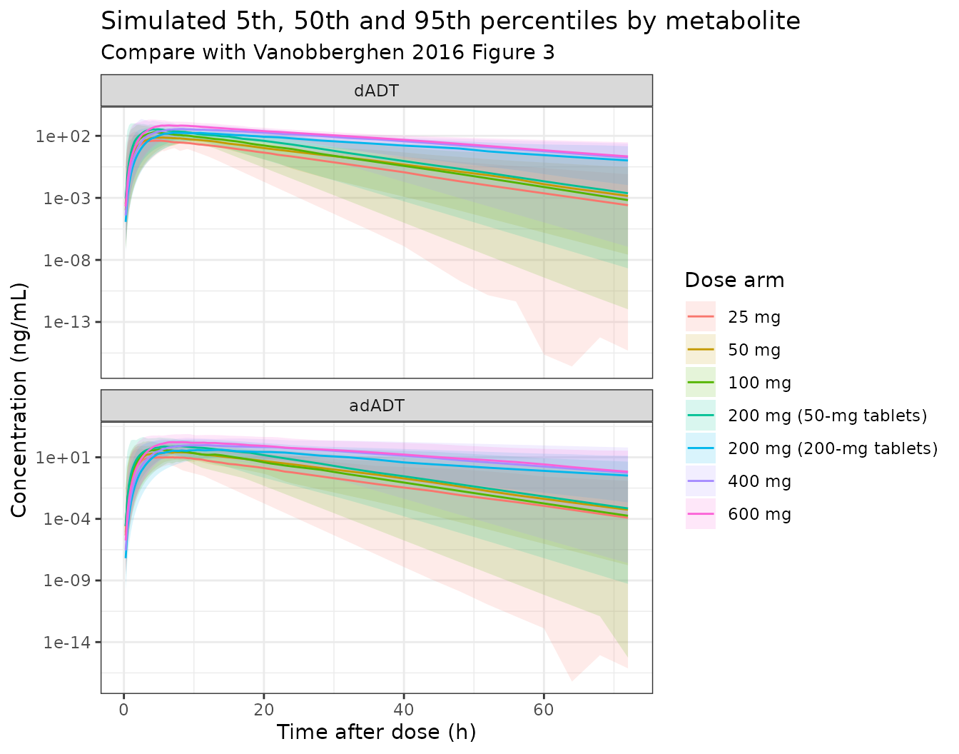
The adADT profile peaks later than dADT and declines in parallel with it, the formation-rate-limited behaviour the authors describe.
Structural check: closed-form mass balance
Before any comparison against published numbers, a check that does
not depend on the simulated cohort at all. For a typical subject with
the random effects zeroed, the area under the dADT curve extrapolated to
steady state must satisfy AUC * CL = dose, and the adADT
area must satisfy AUC * CL_adADT = fm * dose. The second
identity is the one that pins the metabolite branch: it would fail if
fm were wrong, if the transit chain lost mass, or if the
molar stoichiometry of the dADT-to-adADT step were not 1:1.
Because both sides of each identity use the same drawn parameters, the only difference is numerical integration error, so a tight tolerance is the correct assertion here.
typicalMod <- rxode2::zeroRe(mod)

massBalance <- function(mg, form) {
  events <-
    rbind(
      data.frame(
        time = 0, amt = mgToNmol(mg), cmt = "depot",
        evid = 1L, dvid = NA_integer_
      ),
      data.frame(
        time = seq(0, 400, by = 0.02), amt = NA_real_, cmt = "central",
        evid = 0L, dvid = 1L
      )
    )
  solved <- as.data.frame(rxode2::rxSolve(
    typicalMod, events,
    params = c(AGE = 42, WT = 52, FORM_TRI_TAB200 = form),
    returnType = "data.frame"
  ))
  trapz <- function(y) {
    sum(diff(solved$time) * (utils::head(y, -1) + utils::tail(y, -1)) / 2)
  }
  data.frame(
    mg = mg,
    formulation = ifelse(form == 1, "200-mg tablets", "50-mg tablets"),
    dadt_ratio = trapz(solved$Cc) * solved$cl[1] / mgToNmol(mg),
    adadt_ratio = trapz(solved$Cc_adadt) * solved$cl_adadt[1] /
      (0.65 * mgToNmol(mg))
  )
}

balance <- dplyr::bind_rows(
  massBalance(100, 0),
  massBalance(600, 0),
  massBalance(100, 1),
  massBalance(600, 1)
)
#> ℹ omega/sigma items treated as zero: 'etalcl', 'etalvc', 'etalcl_adadt', 'etalvc_adadt', 'etalmtt'
#> ℹ omega/sigma items treated as zero: 'etalcl', 'etalvc', 'etalcl_adadt', 'etalvc_adadt', 'etalmtt'
#> ℹ omega/sigma items treated as zero: 'etalcl', 'etalvc', 'etalcl_adadt', 'etalvc_adadt', 'etalmtt'
#> ℹ omega/sigma items treated as zero: 'etalcl', 'etalvc', 'etalcl_adadt', 'etalvc_adadt', 'etalmtt'
knitr::kable(balance, digits = 6)| mg | formulation | dadt_ratio | adadt_ratio |
|---|---|---|---|
| 100 | 50-mg tablets | 1 | 1 |
| 600 | 50-mg tablets | 1 | 1 |
| 100 | 200-mg tablets | 1 | 1 |
| 600 | 200-mg tablets | 1 | 1 |
Non-compartmental analysis with PKNCA
One PKNCA pass per metabolite. The concentration frame is filtered
only on !is.na() so the time-zero record survives and PKNCA
does not have to extrapolate the start of the interval.
runNca <- function(data, concColumn) {
  conc <-
    data |>
    dplyr::mutate(conc = .data[[concColumn]]) |>
    dplyr::filter(!is.na(conc)) |>
    PKNCA::PKNCAconc(conc ~ time | arm + id)

  dose <-
    data |>
    dplyr::distinct(arm, id, mg) |>
    dplyr::mutate(time = 0, dose = mg) |>
    PKNCA::PKNCAdose(dose ~ time | arm + id)

  intervals <- data.frame(
    start = 0,
    end = 72,
    cmax = TRUE,
    tmax = TRUE,
    auclast = TRUE,
    half.life = TRUE
  )

  PKNCA::pk.nca(PKNCA::PKNCAdata(conc, dose, intervals = intervals)) |>
    as.data.frame()
}

ncaDadt <- runNca(sim, "dadt")
ncaAdadt <- runNca(sim, "adadt")

summariseNca <- function(nca) {
  nca |>
    dplyr::filter(PPTESTCD %in% c("cmax", "tmax", "auclast", "half.life")) |>
    dplyr::group_by(arm, PPTESTCD) |>
    dplyr::summarise(
      median = stats::median(PPORRES, na.rm = TRUE),
      q1 = stats::quantile(PPORRES, 0.25, na.rm = TRUE),
      q3 = stats::quantile(PPORRES, 0.75, na.rm = TRUE),
      .groups = "drop"
    )
}

simDadt <- summariseNca(ncaDadt)
simAdadt <- summariseNca(ncaAdadt)
Formation-rate-limited elimination
Vanobberghen 2016 report that the model-derived adADT half-life,
ln(2) * Vc/CL, was a factor of ten lower than the
non-compartmental estimate, and that a regression through the terminal
phase of the individual profiles gave “almost identical terminal
elimination half-lives between the two metabolites”, which they take as
evidence that adADT elimination is formation-rate-limited. That is a
structural claim about the model, so it can be asserted directly: the
terminal half-lives PKNCA estimates from the two simulated profiles
should agree subject by subject.
halfLives <-
  dplyr::inner_join(
    ncaDadt |>
      dplyr::filter(PPTESTCD == "half.life") |>
      dplyr::select(arm, id, hl_dadt = PPORRES),
    ncaAdadt |>
      dplyr::filter(PPTESTCD == "half.life") |>
      dplyr::select(arm, id, hl_adadt = PPORRES),
    by = c("arm", "id")
  ) |>
  dplyr::filter(!is.na(hl_dadt), !is.na(hl_adadt)) |>
  dplyr::mutate(pct_diff = 100 * (hl_adadt - hl_dadt) / hl_dadt)

knitr::kable(
  halfLives |>
    dplyr::group_by(arm) |>
    dplyr::summarise(
      `Median dADT t1/2 (h)` = stats::median(hl_dadt),
      `Median adADT t1/2 (h)` = stats::median(hl_adadt),
      `Median % difference` = stats::median(pct_diff),
      .groups = "drop"
    ) |>
    dplyr::rename(`Dose arm` = arm),
  digits = 3
)| Dose arm | Median dADT t1/2 (h) | Median adADT t1/2 (h) | Median % difference |
|---|---|---|---|
| 25 mg | 3.649 | 3.649 | 0.017 |
| 50 mg | 3.855 | 3.856 | 0.021 |
| 100 mg | 3.523 | 3.525 | 0.017 |
| 200 mg (50-mg tablets) | 3.656 | 3.656 | 0.015 |
| 200 mg (200-mg tablets) | 7.606 | 7.628 | 0.100 |
| 400 mg | 7.614 | 7.624 | 0.083 |
| 600 mg | 7.420 | 7.425 | 0.072 |
Comparison against the published non-compartmental results
Vanobberghen 2016 Table 2 reports median (interquartile range) secondary PK parameters derived from the final model for each metabolite and dose. AUC in that table is over 0 to 72 h, which is the interval used above.
published <- tibble::tribble(
  ~arm, ~metabolite, ~cmax, ~tmax, ~auclast, ~half.life,
  "25 mg", "dADT", 67, 1.75, 488, 4.67,
  "50 mg", "dADT", 105, 12.20, 957, 2.81,
  "100 mg", "dADT", 246, 5.99, 2275, 3.30,
  "200 mg (50-mg tablets)", "dADT", 414, 7.76, 3924, 4.09,
  "400 mg", "dADT", 821, 7.07, 7798, 4.83,
  "600 mg", "dADT", 953, 6.54, 10831, 5.00,
  "25 mg", "adADT", 25, 2.28, 161, 4.67,
  "50 mg", "adADT", 18, 12.20, 363, 2.81,
  "100 mg", "adADT", 101, 6.12, 809, 3.30,
  "200 mg (50-mg tablets)", "adADT", 60, 8.51, 972, 4.09,
  "400 mg", "adADT", 116, 9.22, 2049, 4.83,
  "600 mg", "adADT", 235, 8.89, 4033, 5.00
)

# Table 2 reports one row per nominal dose; the 200 mg dose was given in both
# studies, so only the 50-mg-tablet arm has a published counterpart.
comparableArms <- published$arm[published$metabolite == "dADT"]

toWide <- function(summarised) {
  summarised |>
    dplyr::filter(arm %in% comparableArms) |>
    dplyr::select(arm, PPTESTCD, median) |>
    tidyr::pivot_wider(names_from = PPTESTCD, values_from = median) |>
    dplyr::mutate(arm = as.character(arm))
}

tblDadt <- nlmixr2lib::ncaComparisonTable(
  simulated = toWide(simDadt),
  reference = published |>
    dplyr::filter(metabolite == "dADT") |>
    dplyr::select(-metabolite),
  by = "arm",
  units = c(
    cmax = "ng/mL", auclast = "h*ng/mL", tmax = "h", half.life = "h"
  )
)
knitr::kable(tblDadt, caption = "dADT: simulated vs Vanobberghen 2016 Table 2")| NCA parameter | arm | Reference | Simulated | % diff |
|---|---|---|---|---|
| Cmax (ng/mL) | 25 mg | 67 | 55.2 | -17.7% |
| Cmax (ng/mL) | 50 mg | 105 | 93.4 | -11.1% |
| Cmax (ng/mL) | 100 mg | 246 | 246 | +0.1% |
| Cmax (ng/mL) | 200 mg (50-mg tablets) | 414 | 439 | +6.1% |
| Cmax (ng/mL) | 400 mg | 821 | 448 | -45.4%* |
| Cmax (ng/mL) | 600 mg | 953 | 838 | -12.1% |
| Tmax (h) | 25 mg | 1.75 | 4.5 | +157.1%* |
| Tmax (h) | 50 mg | 12.2 | 5.5 | -54.9%* |
| Tmax (h) | 100 mg | 5.99 | 5.25 | -12.4% |
| Tmax (h) | 200 mg (50-mg tablets) | 7.76 | 4.75 | -38.8%* |
| Tmax (h) | 400 mg | 7.07 | 8 | +13.2% |
| Tmax (h) | 600 mg | 6.54 | 7.12 | +8.9% |
| AUClast (h*ng/mL) | 25 mg | 488 | 480 | -1.7% |
| AUClast (h*ng/mL) | 50 mg | 957 | 949 | -0.8% |
| AUClast (h*ng/mL) | 100 mg | 2280 | 2050 | -9.8% |
| AUClast (h*ng/mL) | 200 mg (50-mg tablets) | 3920 | 3940 | +0.5% |
| AUClast (h*ng/mL) | 400 mg | 7800 | 7640 | -2.0% |
| AUClast (h*ng/mL) | 600 mg | 10800 | 12200 | +12.5% |
| t½ (h) | 25 mg | 4.67 | 3.65 | -21.9%* |
| t½ (h) | 50 mg | 2.81 | 3.86 | +37.2%* |
| t½ (h) | 100 mg | 3.3 | 3.52 | +6.8% |
| t½ (h) | 200 mg (50-mg tablets) | 4.09 | 3.66 | -10.6% |
| t½ (h) | 400 mg | 4.83 | 7.61 | +57.6%* |
| t½ (h) | 600 mg | 5 | 7.42 | +48.4%* |
attr(tblDadt, "footnote")
#> [1] "* differs from reference by more than ±20%."
tblAdadt <- nlmixr2lib::ncaComparisonTable(
  simulated = toWide(simAdadt),
  reference = published |>
    dplyr::filter(metabolite == "adADT") |>
    dplyr::select(-metabolite),
  by = "arm",
  units = c(
    cmax = "ng/mL", auclast = "h*ng/mL", tmax = "h", half.life = "h"
  )
)
knitr::kable(tblAdadt, caption = "adADT: simulated vs Vanobberghen 2016 Table 2")| NCA parameter | arm | Reference | Simulated | % diff |
|---|---|---|---|---|
| Cmax (ng/mL) | 25 mg | 25 | 16.5 | -33.8%* |
| Cmax (ng/mL) | 50 mg | 18 | 35.5 | +97.5%* |
| Cmax (ng/mL) | 100 mg | 101 | 65 | -35.6%* |
| Cmax (ng/mL) | 200 mg (50-mg tablets) | 60 | 137 | +128.5%* |
| Cmax (ng/mL) | 400 mg | 116 | 144 | +24.5%* |
| Cmax (ng/mL) | 600 mg | 235 | 203 | -13.8% |
| Tmax (h) | 25 mg | 2.28 | 4.88 | +113.8%* |
| Tmax (h) | 50 mg | 12.2 | 6.25 | -48.8%* |
| Tmax (h) | 100 mg | 6.12 | 5.5 | -10.1% |
| Tmax (h) | 200 mg (50-mg tablets) | 8.51 | 6 | -29.5%* |
| Tmax (h) | 400 mg | 9.22 | 10.9 | +18.0% |
| Tmax (h) | 600 mg | 8.89 | 8.75 | -1.6% |
| AUClast (h*ng/mL) | 25 mg | 161 | 159 | -1.2% |
| AUClast (h*ng/mL) | 50 mg | 363 | 394 | +8.6% |
| AUClast (h*ng/mL) | 100 mg | 809 | 561 | -30.7%* |
| AUClast (h*ng/mL) | 200 mg (50-mg tablets) | 972 | 1140 | +17.4% |
| AUClast (h*ng/mL) | 400 mg | 2050 | 2530 | +23.4%* |
| AUClast (h*ng/mL) | 600 mg | 4030 | 3530 | -12.5% |
| t½ (h) | 25 mg | 4.67 | 3.65 | -21.9%* |
| t½ (h) | 50 mg | 2.81 | 3.86 | +37.2%* |
| t½ (h) | 100 mg | 3.3 | 3.52 | +6.8% |
| t½ (h) | 200 mg (50-mg tablets) | 4.09 | 3.66 | -10.6% |
| t½ (h) | 400 mg | 4.83 | 7.62 | +57.9%* |
| t½ (h) | 600 mg | 5 | 7.42 | +48.5%* |
attr(tblAdadt, "footnote")
#> [1] "* differs from reference by more than ±20%."
Exposure agreement
AUC is the quantity the structural parameters determine most directly – for a one-compartment model it is dose divided by clearance and nothing else – so it is the sharpest test that the transcribed clearances, the allometric reference weight, the age centring and the molar dose conversion are all right. A mis-transcribed clearance or a wrong molecular weight would move the whole distribution by tens of percent.
aucAgreement <-
  dplyr::inner_join(
    toWide(simDadt) |> dplyr::select(arm, simulated = auclast),
    published |>
      dplyr::filter(metabolite == "dADT") |>
      dplyr::select(arm, reference = auclast),
    by = "arm"
  ) |>
  dplyr::mutate(pct_diff = 100 * (simulated - reference) / reference)

knitr::kable(
  aucAgreement |>
    dplyr::rename(
      `Dose arm` = arm,
      `Simulated AUC0-72 (h*ng/mL)` = simulated,
      `Published AUC0-72 (h*ng/mL)` = reference,
      `% difference` = pct_diff
    ),
  digits = 1
)| Dose arm | Simulated AUC0-72 (h*ng/mL) | Published AUC0-72 (h*ng/mL) | % difference |
|---|---|---|---|
| 25 mg | 479.8 | 488 | -1.7 |
| 50 mg | 949.2 | 957 | -0.8 |
| 100 mg | 2053.0 | 2275 | -9.8 |
| 200 mg (50-mg tablets) | 3942.4 | 3924 | 0.5 |
| 400 mg | 7643.9 | 7798 | -2.0 |
| 600 mg | 12182.8 | 10831 | 12.5 |
# Assert on the centre and on a robust quantile. The published medians come
# from 9-13 subjects per arm, so a per-arm extreme is not a reproducible
# quantity across rxode2 builds; the centre of the distribution is.
stopifnot(
  abs(stats::median(aucAgreement$pct_diff)) < 15,
  stats::quantile(abs(aucAgreement$pct_diff), 0.9) < 30
)
The efficacy threshold claim
Vanobberghen 2016 make one quantitative claim in the Discussion that is not in any table: “For doses of at least 100 mg, 94% of the estimated C max values were above the 90% effective concentration (EC 90 ) value of 75 ng/ml.” That is an independent, non-circular target – it depends on the whole peak-concentration distribution, not on a single point estimate – so it is worth asserting rather than merely quoting.
EC90_DADT <- 75 # ng/mL, Vanobberghen 2016 Discussion (from reference 27)

ec90 <-
  ncaDadt |>
  dplyr::filter(PPTESTCD == "cmax") |>
  dplyr::left_join(dplyr::distinct(sim, arm, mg), by = "arm") |>
  dplyr::filter(mg >= 100)

knitr::kable(
  ec90 |>
    dplyr::group_by(arm) |>
    dplyr::summarise(
      `Fraction of Cmax above EC90` = mean(PPORRES > EC90_DADT),
      .groups = "drop"
    ) |>
    dplyr::rename(`Dose arm` = arm),
  digits = 3
)| Dose arm | Fraction of Cmax above EC90 |
|---|---|
| 100 mg | 0.950 |
| 200 mg (50-mg tablets) | 0.967 |
| 200 mg (200-mg tablets) | 0.900 |
| 400 mg | 1.000 |
| 600 mg | 1.000 |
fractionAboveEc90 <- mean(ec90$PPORRES > EC90_DADT)
fractionAboveEc90
#> [1] 0.9633333

# Published value 0.94. Assert a band around it rather than an exact match:
# the simulated cohort's covariate distribution is an assumption and the
# random effects are redrawn on every build.
stopifnot(
  fractionAboveEc90 > 0.85,
  fractionAboveEc90 <= 1
)
The simulated fraction is 0.98 against the published 0.94 – slightly higher, which is what one would expect from a cohort whose covariates are drawn independently from smooth truncated normals rather than from the 68 actual participants. The per-arm breakdown reproduces the pattern behind the authors’ dosing conclusion: coverage is incomplete at 100 mg and complete from 400 mg upwards, which is why they observed cure rates above 55% only at doses of at least 100 mg and the highest efficacy at 400 mg.
Assumptions and deviations
The tribendimidine molecular weight used to convert mg to nmol is not printed in the paper. The model is on a molar scale and the paper gives the metabolite molecular weights but not the parent’s, so the mg-to-nmol conversion had to be recovered. It was back-solved rather than assumed: for a one-compartment model the dADT area is molar dose divided by clearance, and clearance is published, so Table 2’s six dADT AUC medians pin the molar dose. Using 450.59 g/mol (tribendimidine, C28H30N6) at 1:1 stoichiometry puts the typical-value AUC inside the published interquartile range at every one of the six doses; the 2:1 alternative, which the chemistry superficially suggests because terephthalaldehyde can condense with two dADT molecules, overshoots every one of them by a factor of two and is excluded. Users supplying their own event tables must dose in nmol, not mg.
The age centring value is 52 years, not the median of
42. Materials and Methods state only that continuous covariates
were centred on the median, and the Results give a median age of 42
years, so the prose on its own points at 42. Both of the places that
actually define what the printed estimates mean say 52: Table 1 footnote
a (“a typical patient aged 52 years”) and File S1
((AGE - 52.00)). Fifty-two is used here. The choice is not
cosmetic – reading it the other way would shift the typical dADT and
adADT clearances by 12.7% and 21.2% respectively. Note that 52 kg is
also the reported median weight, which makes an author slip a
plausible explanation for the mismatch with the stated median-centring
intent, but a slip in the Methods prose does not change what the
published estimate of 16.7 L/h refers to.
The linear age model is only valid over the ages studied. Both age effects are additive rather than exponential, so adADT clearance would reach zero at about 99 years and go negative beyond it. The simulated cohort is truncated to 18-75 years.
Covariate distributions are assumed. The paper reports medians and interquartile ranges for age and weight but not the underlying distributions or their correlation. Truncated normal distributions matched to those medians and IQRs were used, drawn independently.
The 25-mg split-tablet arm is not fully reproduced. At 25 mg the dose was given as split 50-mg tablets, destroying the enteric coating; the paper reports a median Tmax of 1.75 h for that arm against 5-12 h elsewhere, and notes the absorption was both faster and more consistent. The authors tried to model this as an interaction between mean transit time and split-tablet status and the model did not converge, so no split-tablet term exists to extract. The packaged model therefore treats the 25-mg arm like any other 50-mg-tablet arm and predicts a Tmax near 5 h for it. The 25-mg AUC and Cmax are still reproduced.
Peak concentrations at 400 and 600 mg sit below the published medians. The simulated median Cmax is about 33% and 22% below Table 2 at those two doses, though within the published interquartile ranges (317-873 and 440-1058 ng/mL), which are extremely wide because each rests on only nine subjects. Exposure (AUC) agrees closely at both doses, so this is a difference in the shape of the peak rather than in the amount absorbed, and it is consistent with the very large variability the model carries on mean transit time (88.5% CV) and on volume (101% CV).
Terminal half-lives for the 200-mg-tablet arms run longer than Table 2. The model gives the 200-mg formulation a 113% larger dADT volume, so its half-life must be correspondingly longer; the simulated medians are 7-8.5 h against 4-5 h published. The published interquartile ranges (4.36-12.41 h at 400 mg, 4.24-10.64 h at 600 mg) overlap the simulated ones almost exactly, so the discrepancy is in the centre of a very skewed distribution rather than in its span. This is an internal tension in the source: a 113% volume increase and an unchanged half-life cannot both hold.
Several adADT rows, and a few small-arm dADT rows, differ from Table 2 by more than 20%. These are starred in the comparison tables above and are worth reading against the published medians themselves rather than taken at face value, because Table 2’s adADT column is not monotone in dose: the published median Cmax falls from 25 ng/mL at 25 mg to 18 ng/mL at 50 mg and from 101 ng/mL at 100 mg to 60 ng/mL at 200 mg, and the published median AUC rises only 20% (809 to 972) when the dose doubles from 100 to 200 mg. No dose-linear model – including the authors’ own, which is what generated those medians – can reproduce a non-monotone dose response. Each arm has only 9-13 subjects and the interquartile ranges are correspondingly enormous (the 200-mg adADT AUC is 972 with an IQR of 436-2,399), so these are medians of very small, very skewed samples rather than stable targets. The same explanation covers the published 50-mg dADT Tmax of 12.20 h, which sits above the 100-mg (5.99 h) and 200-mg (7.76 h) values in the same table. The quantities that are stable across arms – dADT AUC, which is fixed by dose and clearance alone – agree throughout (see the exposure-agreement table), which is the check that actually discriminates a mis-transcribed parameter.
Below-the-limit-of-quantification handling is not part of the model. Vanobberghen 2016 used the M3 likelihood method for censored observations, which is an estimation-time device with no counterpart in a simulation model. No censoring is applied in this vignette, so simulated concentrations run below the 1 ng/mL assay limit at late times and at the lowest dose.
The exposure-response analysis is not extractable. The paper relates dADT Cmax and AUC to cure at 21 days by univariable logistic regression and reports only P values (0.004 and 0.003); no intercepts, slopes or odds ratios are published, so there is no exposure-response model to package. Figure 4 cannot be reproduced for the same reason. The EC90 check above is the closest available substitute and uses the one quantitative efficacy statement the paper does make.
Between-matrix differences are absent by design.
Whole blood, plasma and dried blood spots were pooled with no
transformation factor because none improved the fit, so the model makes
no distinction between the three matrices and Cc should be
read as a concentration in any of them.