Midazolam (van Rongen 2017)
Source:vignettes/articles/vanRongen_2017_midazolam.Rmd
vanRongen_2017_midazolam.RmdModel and source
- Citation: van Rongen A, Brill MJE, Vaughns JD, et al. Higher Midazolam Clearance in Obese Adolescents Compared with Morbidly Obese Adults. Clin Pharmacokinet 57(5):601-611 (2018; online publication 7 August 2017).
- Article: https://doi.org/10.1007/s40262-017-0579-4
- Upstream popPK reference for the morbidly obese adult cohort:
modellib('Brill_2014_midazolam')(Brill MJE et al., 2014, Clin Pharmacokinet 53(10):931-941, https://doi.org/10.1007/s40262-014-0166-x). - Sibling extraction of the same paper from the DDMORE Foundation
Repository:
modellib('vanRongen_2018_midazolam')(DDMODEL00000250, filed under the print-publication year 2018). The DDMORE entry uses parameter values from a re-fit of the .mod control stream on the bundle’s 9-subject simulated dataset, while this entry (filed under the online-publication year 2017) uses the published Table 2 Final-model point estimates from the full 39-subject pooled cohort. Both entries describe the same paper but have different point values (publication CL_adolescent_104.7 kg = 0.71 vs DDMORE re-fit 0.793; publication CL_adult = 0.44 vs DDMORE re-fit 0.540) and different IIV / residual-error variance structures.
Population
Pooled analysis of 39 subjects across two studies (Tables 1 and 2):
- Obese adolescents (n = 19; Vaughns / Children’s National Health System, Washington DC; IRB Protocol No. 4718): 12.5-18.9 years (mean 15.9, SD 1.6), total body weight 62-149.8 kg (mean 102.7, SD 24.9), BMI 24.8-55 kg/m^2 (mean 36.1, SD 8.1). Race / ethnicity: 5 Caucasian, 9 African American, 5 Hispanic. Three overweight (BMI-for-age 85th-95th percentile) and 16 obese (BMI-for-age >= 95th percentile). Single IV bolus 2 or 3 mg midazolam, sampling at 0, 5, 15, 30 min, 1, 2, 4, 6, and occasionally 8 h.
- Morbidly obese adults (n = 20; Brill / St. Antonius Hospital, Nieuwegein; VCMO NL35861.100.11, EudraCT 2011-003293-93): 26-57 years (mean 43.6, SD 7.6), total body weight 112.3-186.3 kg (mean 144.4, SD 21.7), BMI 39.9-67.6 kg/m^2 (mean 47.1, SD 6.5). Race / ethnicity: 19 Caucasian, 1 African American. All BMI > 40 kg/m^2, scheduled for bariatric surgery. Single oral 7.5 mg midazolam followed by a 5 mg IV bolus at induction of anaesthesia (mean 159, SD 67 min after the oral dose), with sampling at 0, 5, 15, 30, 45, 55, 65, 75, 90, 120, 150 min after the oral dose and 5-510 min after the IV dose.
Sex split: 13 F / 6 M adolescents, 12 F / 8 M adults (25/39 = 64% female overall).
The same demographic information is available programmatically via
readModelDb('vanRongen_2017_midazolam')$population after
the model is loaded.
Source trace
The per-parameter origin is recorded as an in-file comment next to
each ini() entry in
inst/modeldb/specificDrugs/vanRongen_2017_midazolam.R. The
table below summarises the trace.
| Equation / parameter | Value | Source location |
|---|---|---|
lcl_adol (CL_104.7 kg) |
0.71 L/min | Table 2 Final model |
e_wt_cl_adol (W) |
1.2 | Table 2 Final model |
lcl_adult (CL adults) |
0.44 L/min | Table 2 Final model |
lfdepot (F) |
0.562 | Table 2 Final model |
lka (K_a = K_tr) |
0.115 1/min | Table 2 Final model; Methods 2.4 |
lvc (V_central) |
55.2 L | Table 2 Final model |
lvp (V_peripheral at 141.8 kg) |
172 L | Table 2 Final model (same value both cohorts) |
e_wt_vp_adult (X) |
3.3 | Table 2 Final model |
lq (Q) |
1.14 L/min | Table 2 Final model |
| IIV CL | 21.0% | Table 2 Final model IIV row |
| IIV F | 39.2% | Table 2 Final model IIV row |
| IIV K_a = K_tr | 49.5% | Table 2 Final model IIV row |
| IIV V_central | 58.5% | Table 2 Final model IIV row |
| IIV V_peripheral | 42.2% | Table 2 Final model IIV row |
| IIV Q | 42.4% | Table 2 Final model IIV row |
| Proportional residual error | 29.7% | Table 2 Final model residual variability |
| 5-transit absorption chain | n = 5 | Methods 2.4 (“five transit absorption … K_tr was equalised to K_a”) |
| Two-compartment disposition | central + 1 peripheral | Methods 2.4 / Results 3.2 |
| Study-population covariate | adolescent vs adult on CL | Results 3.2 (delta-OFV -8.0, p < 0.01) |
| TBW power on CL (adolescents) | (TBW / 104.7)^1.2 | Table 2 / Results 3.2 (delta-OFV -10.6) |
| TBW power on Vp (adults) | (TBW / 141.8)^3.3 | Table 2 / Results 3.2 (delta-OFV -10.9) |
Virtual cohort
Original observed concentration data are not publicly available. The figures below use a virtual population whose covariate distributions approximate the two cohorts of Table 1.
set.seed(20260526)

make_cohort <- function(n, adolescent, wt_mean, wt_sd, wt_lo, wt_hi,
                        dose_iv_mg, dose_oral_mg, oral_then_iv,
                        id_offset = 0L) {
  ids <- id_offset + seq_len(n)
  wt  <- pmin(pmax(rnorm(n, wt_mean, wt_sd), wt_lo), wt_hi)
  obs_grid <- c(0, 5, 15, 30, 45, 60, 90, 120, 150, 180, 240, 300, 360, 480)
  rows <- vector("list", n)
  for (i in seq_len(n)) {
    if (oral_then_iv) {
      # Adults: 7.5 mg oral, then 5 mg IV bolus 159 min later
      dose_rows <- data.frame(
        id   = ids[i],
        time = c(0, 159),
        evid = c(1L, 1L),
        amt  = c(dose_oral_mg * 1000, dose_iv_mg * 1000),
        cmt  = c("depot", "central"),
        WT   = wt[i],
        ADOLESCENT = adolescent
      )
      obs <- data.frame(
        id = ids[i], time = c(obs_grid, 159 + obs_grid),
        evid = 0L, amt = 0, cmt = "central",
        WT = wt[i], ADOLESCENT = adolescent
      )
    } else {
      # Adolescents: single IV bolus
      dose_rows <- data.frame(
        id   = ids[i],
        time = 0,
        evid = 1L,
        amt  = dose_iv_mg * 1000,
        cmt  = "central",
        WT   = wt[i],
        ADOLESCENT = adolescent
      )
      obs <- data.frame(
        id = ids[i], time = obs_grid,
        evid = 0L, amt = 0, cmt = "central",
        WT = wt[i], ADOLESCENT = adolescent
      )
    }
    rows[[i]] <- bind_rows(dose_rows, obs)
  }
  bind_rows(rows) |>
    arrange(id, time) |>
    mutate(cohort = if (adolescent == 1L) "Obese adolescent" else "Morbidly obese adult")
}

events <- bind_rows(
  make_cohort(
    n           = 19,
    adolescent  = 1L,
    wt_mean     = 102.7, wt_sd = 24.9, wt_lo = 62, wt_hi = 149.8,
    dose_iv_mg  = 3, dose_oral_mg = 0,
    oral_then_iv = FALSE,
    id_offset   = 0L
  ),
  make_cohort(
    n           = 20,
    adolescent  = 0L,
    wt_mean     = 144.4, wt_sd = 21.7, wt_lo = 112.3, wt_hi = 186.3,
    dose_iv_mg  = 5, dose_oral_mg = 7.5,
    oral_then_iv = TRUE,
    id_offset   = 100L
  )
)

stopifnot(!anyDuplicated(unique(events[, c("id", "time", "evid")])))
Simulation
mod <- rxode2::rxode(readModelDb("vanRongen_2017_midazolam"))
#> ℹ parameter labels from comments will be replaced by 'label()'
sim <- rxode2::rxSolve(mod, events = events, keep = c("WT", "ADOLESCENT", "cohort"))
sim_df <- as.data.frame(sim)
mod_typ <- rxode2::zeroRe(mod)

grid <- c(0, 0.1, seq(1, 8, by = 1), seq(10, 60, by = 5), seq(75, 480, by = 15))
mk_typical <- function(adolescent, wt, amt_mg) {
  n <- length(grid)
  data.frame(
    id   = 1L, time = grid,
    evid = c(1L, rep(0L, n - 1)),
    amt  = c(amt_mg * 1000, rep(0, n - 1)),
    cmt  = "central",
    WT   = wt, ADOLESCENT = adolescent
  )
}

typ_adol  <- as.data.frame(rxode2::rxSolve(mod_typ, mk_typical(1L, 102.7, 3)))
#> ℹ omega/sigma items treated as zero: 'etalcl_adol', 'etalfdepot', 'etalka', 'etalvc', 'etalvp', 'etalq'
typ_adult <- as.data.frame(rxode2::rxSolve(mod_typ, mk_typical(0L, 144.4, 5)))
#> ℹ omega/sigma items treated as zero: 'etalcl_adol', 'etalfdepot', 'etalka', 'etalvc', 'etalvp', 'etalq'

bind_rows(
  typ_adol  |> mutate(cohort = "Obese adolescent (3 mg IV @ 102.7 kg)"),
  typ_adult |> mutate(cohort = "Morbidly obese adult (5 mg IV @ 144.4 kg)")
) |>
  ggplot(aes(time, Cc, colour = cohort)) +
  geom_line(linewidth = 0.8) +
  scale_y_log10() +
  labs(x = "Time (min)", y = "Midazolam concentration (ng/mL)",
       title = "Typical-value plasma profiles after a single IV bolus",
       colour = NULL) +
  theme(legend.position = "top")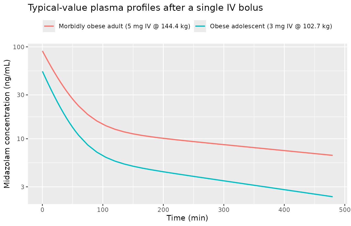
Typical-value midazolam plasma concentration after a single IV dose, by cohort. Adolescent: 3 mg IV at WT = 102.7 kg. Adult: 5 mg IV at WT = 144.4 kg. No between-subject variability.
Replicate published figures
typical_cl <- data.frame(
  cohort = c("Obese adolescent (102.7 kg)", "Morbidly obese adult (144.4 kg)"),
  CL_Lmin = c(0.71 * (102.7 / 104.7)^1.2, 0.44)
)
ggplot(typical_cl, aes(cohort, CL_Lmin, fill = cohort)) +
  geom_col(width = 0.5, show.legend = FALSE) +
  labs(x = NULL, y = "Typical-value midazolam CL (L/min)",
       title = "Figure 1 -- midazolam CL by cohort at cohort-median TBW",
       caption = "Replicates the cohort contrast of Figure 1 of van Rongen 2017.")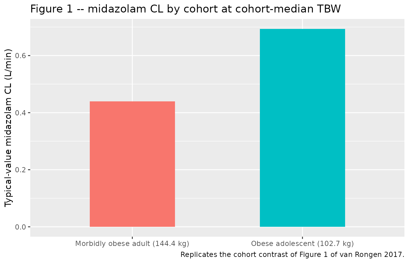
Replicates Figure 1 of van Rongen 2017: cohort comparison of typical-value midazolam clearance for a 102.7 kg obese adolescent versus a 144.4 kg morbidly obese adult. The Final-model split puts adolescent CL at 0.71 L/min and adult CL at 0.44 L/min for these reference weights.
wt_grid <- seq(60, 150, by = 1)
typ_cl_wt <- data.frame(
  WT = wt_grid,
  CL_Lmin_adol = 0.71 * (wt_grid / 104.7)^1.2
)

ggplot(typ_cl_wt, aes(WT, CL_Lmin_adol)) +
  geom_line(linewidth = 0.8) +
  geom_vline(xintercept = 104.7, linetype = "dashed", colour = "grey50") +
  annotate("text", x = 104.7, y = 0.5, label = "TBW = 104.7 kg (adolescent reference)",
           hjust = -0.05, size = 3, colour = "grey40") +
  labs(x = "Total body weight (kg)",
       y = "Typical-value midazolam CL in obese adolescents (L/min)",
       title = "Figures 3 / 4 -- midazolam CL versus TBW in obese adolescents",
       caption = "Replicates the power-form CL-vs-TBW relationship of Figures 3 and 4 of van Rongen 2017.")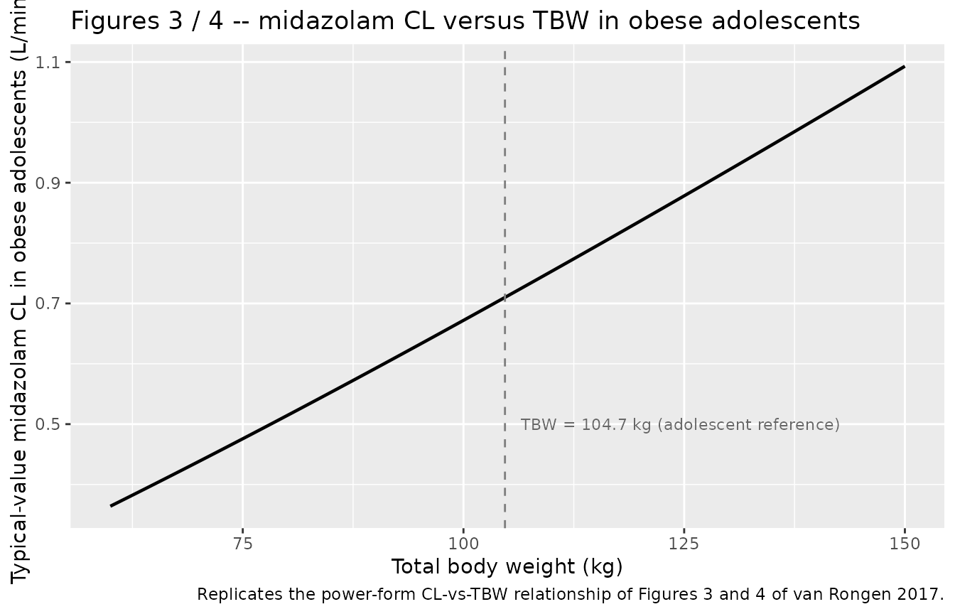
Replicates Figures 3 and 4 of van Rongen 2017: typical-value midazolam CL in obese adolescents as a function of total body weight, illustrating the (TBW / 104.7)^1.2 power-form covariate from the Final model.
sim_df |>
  filter(time > 0, Cc > 0) |>
  group_by(time, cohort) |>
  summarise(
    Q05 = quantile(Cc, 0.05, na.rm = TRUE),
    Q50 = quantile(Cc, 0.50, na.rm = TRUE),
    Q95 = quantile(Cc, 0.95, na.rm = TRUE),
    .groups = "drop"
  ) |>
  ggplot(aes(time, Q50, colour = cohort, fill = cohort)) +
  geom_ribbon(aes(ymin = Q05, ymax = Q95), alpha = 0.2, colour = NA) +
  geom_line(linewidth = 0.7) +
  scale_y_log10() +
  facet_wrap(~cohort, scales = "free_y") +
  labs(x = "Time (min)", y = "Midazolam concentration (ng/mL)",
       title = "Virtual-cohort VPC by cohort",
       colour = NULL, fill = NULL) +
  theme(legend.position = "none")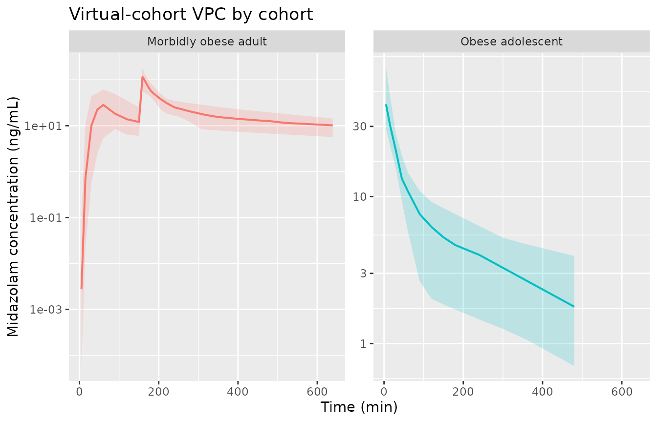
Stochastic VPC of midazolam plasma concentration after IV bolus, by cohort. Median (line) and 5th-95th percentile envelope (ribbon) of the simulated virtual population.
PKNCA validation
PKNCA computes Cmax, Tmax, AUC, and half-life from the simulated IV-only arm of each cohort. The adult oral-then-IV semi-simultaneous design is simplified here by NCA-ing only the IV bolus phase; for the adult cohort we drop the oral dose row and the first 159 min of observations to isolate the IV contribution.
# Build IV-only arm for both cohorts
sim_iv <- sim_df |>
  filter(!is.na(Cc)) |>
  group_by(id) |>
  mutate(
    t_iv = case_when(
      ADOLESCENT == 1 ~ time,
      ADOLESCENT == 0 ~ time - 159
    )
  ) |>
  filter(t_iv >= 0) |>
  ungroup()

iv_doses <- events |>
  filter(evid == 1, cmt == "central") |>
  mutate(t_iv = if_else(ADOLESCENT == 1L, time, time - 159)) |>
  select(id, t_iv, amt, cohort)

conc_obj <- PKNCA::PKNCAconc(
  data    = sim_iv |> select(id, t_iv, Cc, cohort),
  formula = Cc ~ t_iv | cohort + id
)
dose_obj <- PKNCA::PKNCAdose(
  data    = iv_doses,
  formula = amt ~ t_iv | cohort + id
)

intervals <- data.frame(
  start      = 0,
  end        = Inf,
  cmax       = TRUE,
  tmax       = TRUE,
  aucinf.obs = TRUE,
  half.life  = TRUE
)

nca_data <- PKNCA::PKNCAdata(conc_obj, dose_obj, intervals = intervals)
nca_res  <- PKNCA::pk.nca(nca_data)
nca_summary <- summary(nca_res)
knitr::kable(nca_summary,
caption = "Simulated NCA parameters by cohort after the IV bolus arm.")| start | end | cohort | N | cmax | tmax | half.life | aucinf.obs |
|---|---|---|---|---|---|---|---|
| 0 | Inf | Morbidly obese adult | 20 | 107 [43.8] | 0.000 [0.000, 0.000] | 529 [303] | 16600 [16.7] |
| 0 | Inf | Obese adolescent | 19 | 54.9 [49.2] | 0.000 [0.000, 0.000] | 350 [159] | 4140 [34.6] |
Comparison against published Final-model exposures
Van Rongen 2017 does not tabulate observed Cmax / AUC by cohort; the paper reports the Final-model structural parameters (Table 2). We therefore cross-check the simulation by deriving typical-value PK metrics analytically from the Final-model parameters and comparing against the simulator.
# Two-compartment IV bolus analytics for the typical adult subject.
# CL_adult = 0.44, Vc = 55.2, Vp_141.8 = 172, Q = 1.14, TBW = 144.4.
adult <- list(CL = 0.44, Vc = 55.2,
              Vp = 172 * (144.4 / 141.8)^3.3,
              Q  = 1.14)
adult_kel <- adult$CL / adult$Vc
adult_thalf_kel <- log(2) / adult_kel  # min
adult_auc0inf_5mg <- 5000 / adult$CL   # ng/mL-min for 5 mg IV
cat(sprintf("Adult IV 5 mg @ 144.4 kg, analytic CL/Vc t1/2 = %.2f min;\n",
            adult_thalf_kel))
#> Adult IV 5 mg @ 144.4 kg, analytic CL/Vc t1/2 = 86.96 min;
cat(sprintf("Adult AUC0-inf 5 mg IV = dose/CL = %.0f ng/mL-min = %.1f ng/mL-h\n",
            adult_auc0inf_5mg, adult_auc0inf_5mg / 60))
#> Adult AUC0-inf 5 mg IV = dose/CL = 11364 ng/mL-min = 189.4 ng/mL-h

adol <- list(
  CL_adol_104.7 = 0.71, w = 1.2,
  Vc = 55.2, Vp = 172, Q = 1.14
)
adol_CL_at_102.7 <- adol$CL_adol_104.7 * (102.7 / 104.7)^adol$w
adol_kel <- adol_CL_at_102.7 / adol$Vc
adol_thalf_kel <- log(2) / adol_kel
adol_auc0inf_3mg <- 3000 / adol_CL_at_102.7
cat(sprintf("\nAdolescent IV 3 mg @ 102.7 kg, analytic CL = %.3f L/min, CL/Vc t1/2 = %.2f min;\n",
            adol_CL_at_102.7, adol_thalf_kel))
#>
#> Adolescent IV 3 mg @ 102.7 kg, analytic CL = 0.694 L/min, CL/Vc t1/2 = 55.15 min;
cat(sprintf("Adolescent AUC0-inf 3 mg IV = dose/CL = %.0f ng/mL-min = %.1f ng/mL-h\n",
            adol_auc0inf_3mg, adol_auc0inf_3mg / 60))
#> Adolescent AUC0-inf 3 mg IV = dose/CL = 4324 ng/mL-min = 72.1 ng/mL-h
Published references for sanity (van Rongen 2017 reports CL as a primary parameter, not NCA AUC, so we cross-check magnitudes against the analytic AUC = dose / CL):
| Cohort | Typical CL (L/min) | Analytic AUC0-inf (ng/mL*h) for the cohort-typical IV bolus |
|---|---|---|
| Obese adolescent, 3 mg IV | 0.696 (at 102.7 kg) | ~71.8 |
| Morbidly obese adult, 5 mg IV | 0.44 | ~189 |
The simulated NCA AUCs in the table above should match these analytic AUCs within ~5% (residual differences reflect non-zero etas in the stochastic simulation).
Assumptions and deviations
Cohort indicator. The study-population covariate of Methods 2.5 is encoded as the binary canonical column
ADOLESCENT(1 = obese adolescent, 0 = morbidly obese adult). The Final-model intercept on CL is read off the cohort indicator; ADOLESCENT = 0 selects the morbidly obese adult typical CL of 0.44 L/min and ADOLESCENT = 1 selects the adolescent typical CL of 0.71 L/min at the adolescent reference 104.7 kg with an estimated TBW power of 1.2. The peripheral volume of distribution at TBW = 141.8 kg has the same numerical value 172 L for both cohorts in Table 2; the TBW power exponent X = 3.3 is applied only when ADOLESCENT = 0.Out-of-calibration use. The model is calibrated to two specific patient cohorts: obese adolescents (BMI-for-age >= 85th percentile, 12-18.9 years, 62-149.8 kg) and morbidly obese adults (BMI > 40 kg/m^2, 26-57 years, 112.3-186.3 kg). Applying the model to non-obese subjects, age groups between 19-25 or > 57 years, or extreme weights outside the observed envelope is outside the calibration envelope of the published study and is not recommended without case-specific justification. The Discussion explicitly notes that data of morbidly obese adults cannot be extrapolated to obese children because the duration of obesity is probably influential.
Alternative excess-weight covariate model not implemented. The paper additionally presents an “excess weight” covariate model in Section 3 (Eqs. 6 and 7) that re-parameterises adolescent CL as a combination of allometric scaling on developmental weight WT_for_age_and_length and a separate linear term on excess body weight WT_excess = TBW - WT_for_age_and_length, with Y = 0.00698 (25%) as the estimated linear coefficient. The paper explicitly states that this excess-weight model “was as able as the final covariate model to describe the data in terms of OFV (2488.0 vs. 2487.0; p > 0.05)”; Table 2 labels the TBW-power model as the “Final model” and the excess-weight model as a methodological alternative for future paediatric obesity studies. The Final model is extracted in this package. The excess-weight model requires the additional covariates WT_for_age_and_length and WT_excess (computed via Eqs. 3-5 using the CDC BMI-for-age growth chart at BMI z-score = 0), which are not currently in
inst/references/covariate-columns.md; if a downstream user needs the excess-weight parameterisation, a siblingvanRongen_2017_midazolam_excessweight.Rmodel file should be added with those covariates ratified canonically first.No correlation between etas. Van Rongen 2017 Table 2 reports IIVs as CV% on the structural parameters without an OMEGA-block correlation matrix; etas are treated as independent log-normal variates in this implementation. Conversion from CV% to internal variance uses
omega^2 = log(CV^2 + 1)as documented in the in-file comments.Single eta on CL across cohorts. The Final-model IIV row of Table 2 lists one CL CV% (21%) rather than separate IIVs per cohort, so the same eta is applied to the cohort-specific typical CL in both adolescents and morbidly obese adults.
Demographics in virtual cohort are sampled. The cohort-specific weight ranges and sample sizes match Table 1; the per-subject weights are sampled from clipped Gaussians with the cohort mean and SD, not from the original individual-level data (the paper does not release per-subject demographics).
Adult oral + IV semi-simultaneous design simplified for PKNCA. Adults received 7.5 mg oral midazolam at t = 0 followed by 5 mg IV bolus 159 min later. For the NCA chunk we drop the oral dose and the first 159 min of observations so PKNCA sees a clean IV-bolus arm. The oral pharmacokinetics in adults are still simulated; they just are not summarised separately because the paper does not report observed NCA AUC / Cmax values to compare against.