Sufentanil, epidural (Bienert 2025)
Source:vignettes/articles/Bienert_2025_sufentanil.Rmd
Bienert_2025_sufentanil.RmdModel and source
- Citation: Bienert A, Borsuk-De Moor A, Okunska P, Ber J, Siluk D, Waszczuk M, Kusza K, Bartkowiak T, Szrama J, Kluzik A, Koszel T, Wiczling P. Pharmacokinetics of Sufentanil After Epidural Administration During the Course of Extensive Abdominal Surgery. Clin Pharmacokinet 2025;64(9):1331-1340. doi:10.1007/s40262-025-01543-y. Correlations of the random effects are from the authors’ public code and output deposit (https://github.com/wiczling/sufentanil-epidural, deliv/tables/torsten/3b/parameters-table.csv) for the same final model.
- Description: Two-compartment population PK model for epidural sufentanil in adults undergoing major abdominal surgery under general anaesthesia with epidural analgesia (epidural bolus plus continuous epidural infusion for up to about 3 days). Absorption from the epidural space is itself two-compartmental: the dose enters an epidural absorption compartment that drains first order into plasma (KA) and exchanges with a slowly returning epidural distribution compartment (epidural fat; KA14 out, KA41 back), which produces flip-flop kinetics. Linear elimination from the central compartment. Full Bayesian fit (Stan/Torsten); typical values are posterior means. Log-normal IIV on all seven parameters with a full correlation matrix; residual error additive on the log scale with a Student-t distribution.
- Article: Clin Pharmacokinet 2025;64(9):1331-1340
Sufentanil given into the epidural space reaches plasma slowly, and
its plasma concentrations decline more slowly than after intravenous
dosing. Bienert 2025 explains this with a two-compartment absorption
site: the dose enters an epidural absorption compartment
(depot, the paper’s A1) that drains quickly into plasma
(KA) and also exchanges quickly with an epidural distribution
compartment (depot_peripheral, the paper’s A4, attributed
to epidural fat) from which sufentanil returns only slowly (KA41).
Disposition is a standard two-compartment model. Because the slow return
from the epidural fat is slower than sufentanil’s own terminal
disposition, the post-infusion decline is absorption-limited (flip-flop
kinetics).
mod <- rxode2::rxode(readModelDb("Bienert_2025_sufentanil"))
#> ℹ parameter labels from comments will be replaced by 'label()'
mod
#>  ── rxode2-based free-form 4-cmt ODE model ──────────────────────────────────────
#>  ── Initalization: ──
#> Fixed Effects ($theta):
#>       lcl        lq       lvc       lvp       lka     lka14     lka41     expSd
#>  4.172848  3.875359  2.322388  6.226537  1.184790  2.701361 -1.966113  0.310000
#>        nu
#>  3.810000
#>
#> Omega ($omega):
#>               etalcl        etalq       etalvc       etalvp       etalka
#> etalcl    0.24010000  0.006945750  0.187194700 -0.003616200 -0.002205000
#> etalq     0.00694575  0.202500000 -0.028674900  0.000440955  0.002980800
#> etalvc    0.18719470 -0.028674900  2.280100000 -0.027921410  0.001723212
#> etalvp   -0.00361620  0.000440955 -0.027921410  0.168100000  0.003808080
#> etalka   -0.00220500  0.002980800  0.001723212  0.003808080  0.129600000
#> etalka14  0.00465500  0.003471300 -0.054797900 -0.003739200  0.010369440
#> etalka41  0.04581500  0.023850000  0.083805000 -0.007277500 -0.014598000
#>             etalka14   etalka41
#> etalcl    0.00465500  0.0458150
#> etalq     0.00347130  0.0238500
#> etalvc   -0.05479790  0.0838050
#> etalvp   -0.00373920 -0.0072775
#> etalka    0.01036944 -0.0145980
#> etalka14  0.14440000  0.0212800
#> etalka41  0.02128000  0.2500000
#> attr(,"lotriLabels")
#> [1] NA
#> [2] NA
#> [3] NA
#> [4] NA
#> [5] NA
#> [6] NA
#> [7] "Table 1: omegaCL 0.49, omegaQ 0.45, omegaV1 1.51, omegaV2 0.41, omegaKA 0.36, omegaKA14 0.38, omegaKA41 0.5; rho from the deposited parameters-table.csv"
#> attr(,"lotriFix")
#>          etalcl etalq etalvc etalvp etalka etalka14 etalka41
#> etalcl    FALSE FALSE  FALSE  FALSE  FALSE    FALSE    FALSE
#> etalq     FALSE FALSE  FALSE  FALSE  FALSE    FALSE    FALSE
#> etalvc    FALSE FALSE  FALSE  FALSE  FALSE    FALSE    FALSE
#> etalvp    FALSE FALSE  FALSE  FALSE  FALSE    FALSE    FALSE
#> etalka    FALSE FALSE  FALSE  FALSE  FALSE    FALSE    FALSE
#> etalka14  FALSE FALSE  FALSE  FALSE  FALSE    FALSE    FALSE
#> etalka41  FALSE FALSE  FALSE  FALSE  FALSE    FALSE    FALSE
#>
#> States ($state or $stateDf):
#>   Compartment Number Compartment Name
#> 1                  1            depot
#> 2                  2 depot_peripheral
#> 3                  3          central
#> 4                  4      peripheral1
#>  ── μ-referencing ($muRefTable): ──
#>   theta      eta level
#> 1   lcl   etalcl    id
#> 2    lq    etalq    id
#> 3   lvc   etalvc    id
#> 4   lvp   etalvp    id
#> 5   lka   etalka    id
#> 6 lka14 etalka14    id
#> 7 lka41 etalka41    id
#>
#>  ── Model (Normalized Syntax): ──
#> function() {
#>     compartmentData <- list(depot = list(analyte = "sufentanil",
#>         units = "ug", specimen = "administration site", verified = TRUE),
#>         depot_peripheral = list(analyte = "sufentanil", units = "ug",
#>             specimen = "administration site", verified = TRUE),
#>         central = list(analyte = "sufentanil", units = "ug",
#>             specimen = "plasma", verified = TRUE), peripheral1 = list(analyte = "sufentanil",
#>             units = "ug", specimen = "plasma", verified = TRUE))
#>     covariateData <- list()
#>     covariatesDataExcluded <- list(AGE = list(description = "Age",
#>         units = "years", type = "continuous", notes = "Explored graphically against the individual random effects (Figure S5); no covariate model was fitted."),
#>         WT = list(description = "Body weight", units = "kg",
#>             type = "continuous", notes = "Explored graphically against the individual random effects (Figure S6); no covariate model was fitted."),
#>         HT = list(description = "Body height", units = "cm",
#>             type = "continuous", notes = "Explored graphically against the individual random effects (Figure S7); no covariate model was fitted."),
#>         SEXF = list(description = "Sex (1 = female, 0 = male)",
#>             units = "(binary)", type = "binary", notes = "Explored graphically against the individual random effects (Figure S8); no covariate model was fitted."))
#>     description <- "Two-compartment population PK model for epidural sufentanil in adults undergoing major abdominal surgery under general anaesthesia with epidural analgesia (epidural bolus plus continuous epidural infusion for up to about 3 days). Absorption from the epidural space is itself two-compartmental: the dose enters an epidural absorption compartment that drains first order into plasma (KA) and exchanges with a slowly returning epidural distribution compartment (epidural fat; KA14 out, KA41 back), which produces flip-flop kinetics. Linear elimination from the central compartment. Full Bayesian fit (Stan/Torsten); typical values are posterior means. Log-normal IIV on all seven parameters with a full correlation matrix; residual error additive on the log scale with a Student-t distribution."
#>     dosing <- "depot"
#>     paper_specific_compartments <- "depot_peripheral"
#>     population <- list(species = "human", n_subjects = 23L, n_studies = 1L,
#>         age_range = "30-83 years", age_median = "60 years (IQR 42.5-65)",
#>         weight_median = "71 kg (IQR 59-80.5)", sex_female_pct = 52,
#>         disease_state = "Adults (ASA physical status 2-3) undergoing major oncologic or non-oncologic abdominal surgery under general anaesthesia combined with epidural analgesia (epidural catheter at Th8/9 to Th12/L1).",
#>         dose_range = "Epidural sufentanil: an initial dose with an amide local anaesthetic (ropivacaine or bupivacaine), followed by a continuous epidural infusion titrated to clinical response during surgery and for the following 3 days. Median (IQR) total intra-operative epidural sufentanil dose 15 (10.9-20.6) ug (Table S1).",
#>         regions = "Poland (single centre, Poznan University of Medical Sciences)",
#>         notes = "Study NCT06069219. Demographics from Tables S1 and S2: 12 female / 11 male; ASA 2 in 9 and ASA 3 in 14 patients; general anaesthesia with sevoflurane (20) or desflurane (3) after IV fentanyl and propofol induction. Plasma sampled at 5 min, 0.5, 1, 2, 4, 6 and 12 h, then every 24 h, before the end of infusion, and at 3, 5, 20 and 40 min and 1, 2, 6, 12, 36 and 72 h after the infusion ended; LC-MS/MS assay. Two very high concentrations just after the start of the infusion were flagged as outliers (Figure 2). Stan/Torsten full Bayesian estimation, 4 chains x 1000 post-warmup iterations, weakly informative priors on disposition taken from published IV sufentanil PK.")
#>     reference <- "Bienert A, Borsuk-De Moor A, Okunska P, Ber J, Siluk D, Waszczuk M, Kusza K, Bartkowiak T, Szrama J, Kluzik A, Koszel T, Wiczling P. Pharmacokinetics of Sufentanil After Epidural Administration During the Course of Extensive Abdominal Surgery. Clin Pharmacokinet 2025;64(9):1331-1340. doi:10.1007/s40262-025-01543-y. Correlations of the random effects are from the authors' public code and output deposit (https://github.com/wiczling/sufentanil-epidural, deliv/tables/torsten/3b/parameters-table.csv) for the same final model."
#>     units <- list(time = "h", dosing = "ug", concentration = "pg/mL")
#>     vignette <- "Bienert_2025_sufentanil"
#>     ini({
#>         lcl <- 4.17284762371004
#>         label("Clearance (L/h)")
#>         lq <- 3.87535902105655
#>         label("Inter-compartmental clearance (L/h)")
#>         lvc <- 2.32238772029023
#>         label("Central volume of distribution (L)")
#>         lvp <- 6.22653666928747
#>         label("Peripheral volume of distribution (L)")
#>         lka <- 1.18478998490916
#>         label("Absorption rate constant, epidural space to plasma (1/h)")
#>         lka14 <- 2.70136121295141
#>         label("Rate constant, epidural absorption to epidural distribution compartment (1/h)")
#>         lka41 <- -1.96611285637283
#>         label("Rate constant, epidural distribution compartment back to epidural absorption compartment (1/h)")
#>         expSd <- c(0, 0.31)
#>         label("Residual scale on the log concentration (Student-t)")
#>         nu <- c(0, 3.81)
#>         label("Degrees of freedom of the Student-t residual error")
#>         etalcl ~ c(etalcl = 0.2401)
#>         etalq ~ c(etalcl = 0.00694575, etalq = 0.2025)
#>         etalvc ~ c(etalcl = 0.1871947, etalq = -0.0286749, etalvc = 2.2801)
#>         etalvp ~ c(etalcl = -0.0036162, etalq = 0.000440955,
#>             etalvc = -0.02792141, etalvp = 0.1681)
#>         etalka ~ c(etalcl = -0.002205, etalq = 0.0029808, etalvc = 0.001723212,
#>             etalvp = 0.00380808, etalka = 0.1296)
#>         etalka14 ~ c(etalcl = 0.004655, etalq = 0.0034713, etalvc = -0.0547979,
#>             etalvp = -0.0037392, etalka = 0.01036944, etalka14 = 0.1444)
#>         etalka41 ~ c(etalcl = 0.045815, etalq = 0.02385, etalvc = 0.083805,
#>             etalvp = -0.0072775, etalka = -0.014598, etalka14 = 0.02128,
#>             etalka41 = 0.25)
#>         label("Table 1: omegaCL 0.49, omegaQ 0.45, omegaV1 1.51, omegaV2 0.41, omegaKA 0.36, omegaKA14 0.38, omegaKA41 0.5; rho from the deposited parameters-table.csv")
#>     })
#>     model({
#>         cl <- exp(lcl + etalcl)
#>         q <- exp(lq + etalq)
#>         vc <- exp(lvc + etalvc)
#>         vp <- exp(lvp + etalvp)
#>         ka <- exp(lka + etalka)
#>         ka14 <- exp(lka14 + etalka14)
#>         ka41 <- exp(lka41 + etalka41)
#>         kel <- cl/vc
#>         k12 <- q/vc
#>         k21 <- q/vp
#>         d/dt(depot) <- -(ka + ka14) * depot + ka41 * depot_peripheral
#>         d/dt(depot_peripheral) <- ka14 * depot - ka41 * depot_peripheral
#>         d/dt(central) <- ka * depot - (kel + k12) * central +
#>             k21 * peripheral1
#>         d/dt(peripheral1) <- k12 * central - k21 * peripheral1
#>         Cc <- 1000 * central/vc
#>         Cc ~ lnorm(expSd) + dt(nu)
#>     })
#> }
Population
Bienert 2025 studied 23 adults (12 female, 11 male; ASA physical status 2 in 9 and 3 in 14 patients) undergoing major oncologic or non-oncologic abdominal surgery under general anaesthesia combined with epidural analgesia at a single centre in Poznan, Poland (NCT06069219). The abstract gives an age range of 30-83 years; Table S1 reports a median (IQR) age of 60 (42.5-65) years and body weight of 71 (59-80.5) kg. The epidural catheter sat between Th8/9 and Th12/L1. After an initial epidural dose of sufentanil with an amide local anaesthetic, sufentanil was infused epidurally, titrated to response, during surgery and for the following 3 days (median intra-operative epidural dose 15 ug, Table S1). Plasma was sampled densely during the infusion and for 72 h after it stopped.
Age, weight, height, sex and catheter placement were explored only graphically against the individual random effects (Figures S5-S9); no covariate model was fitted, so the model has no covariates.
pop <- mod$population
str(pop[c("species", "n_subjects", "age_range", "age_median", "weight_median", "sex_female_pct")])
#> List of 6
#>  $ species       : chr "human"
#>  $ n_subjects    : int 23
#>  $ age_range     : chr "30-83 years"
#>  $ age_median    : chr "60 years (IQR 42.5-65)"
#>  $ weight_median : chr "71 kg (IQR 59-80.5)"
#>  $ sex_female_pct: num 52
Source trace
| Item | Value | Source |
|---|---|---|
| ODE system (A1, A4, C1, C2) | as in model()
|
Statistical Methods, final model equations; K matrix of the
deposited Stan code (model/torsten/3b/3b.stan) |
| Concentration = amount / V1 x 1000 (pg/mL) | Deposited Stan code (x[2] ./ theta[3] .* 1000) |
|
lcl |
64.9 L/h | Table 1, thetaCL mean |
lq |
48.2 L/h | Table 1, thetaQ mean |
lvc |
10.2 L | Table 1, thetaV1 mean |
lvp |
506 L | Table 1, thetaV2 mean |
lka |
3.27 1/h | Table 1, thetaKA mean |
lka14 |
14.9 1/h | Table 1, thetaKA14 mean |
lka41 |
0.14 1/h | Table 1, thetaKA41 mean |
| IIV SDs (log scale) | 0.49, 0.45, 1.51, 0.41, 0.36, 0.38, 0.5 | Table 1, omega CL, Q, V1, V2, KA, KA14, KA41 means |
| IIV correlations | 21 posterior-mean rho | Deposited
deliv/tables/torsten/3b/parameters-table.csv
|
| Omega = diag(omega) rho diag(omega) | Statistical Methods | |
expSd |
0.31 | Table 1, sigma mean |
nu |
3.81 | Table 1, nu mean |
| Student-t residual on log(C) | Statistical Methods |
Replicating Figure S10: dosing to an epidural steady state
The Discussion derives a regimen that puts the epidural absorption
compartment at its steady-state amount from the start: an induction dose
of Rss / KA followed by an infusion whose rate decays as
Rss + KA14 / KA * Rss * exp(-KA41 * t). With that input,
depot holds exactly at Rss / KA (the KA14
outflow is replaced by the decaying extra rate) while the epidural fat
fills, and plasma approaches Rss / CL. Figure S10 shows
this for Rss = 3 ug/h in the typical subject. The decaying
rate is given here as consecutive 0.05-h infusions, each carrying the
exact integral of the rate over its interval.
typ <- rxode2::zeroRe(mod)
ka <- exp(mod$theta[["lka"]])
ka14 <- exp(mod$theta[["lka14"]])
ka41 <- exp(mod$theta[["lka41"]])
cl <- exp(mod$theta[["lcl"]])
rss <- 3
dt_seg <- 0.05
t_seg <- seq(0, 72 - dt_seg, by = dt_seg)
seg_amt <- rss * dt_seg +
  (ka14 / ka) * rss / ka41 * (exp(-ka41 * t_seg) - exp(-ka41 * (t_seg + dt_seg)))

ev_s10 <- dplyr::bind_rows(
  data.frame(id = 1L, time = 0, amt = rss / ka, rate = 0, evid = 1L, cmt = "depot"),
  data.frame(id = 1L, time = t_seg, amt = seg_amt, rate = seg_amt / dt_seg, evid = 1L, cmt = "depot"),
  data.frame(id = 1L, time = seq(0, 72, by = 0.25), amt = 0, rate = 0, evid = 0L, cmt = "central")
)
sim_s10 <- rxode2::rxSolve(typ, ev_s10, atol = 1e-10, rtol = 1e-10) |>
  as.data.frame()
#> ℹ omega/sigma items treated as zero: 'etalcl', 'etalq', 'etalvc', 'etalvp', 'etalka', 'etalka14', 'etalka41'

rate_df <- data.frame(time = seq(0, 72, by = 0.25)) |>
  dplyr::mutate(value = rss + (ka14 / ka) * rss * exp(-ka41 * time), panel = "Infusion rate (ug/h)")
plot_s10 <- dplyr::bind_rows(
  rate_df,
  sim_s10 |> dplyr::transmute(time, value = depot, panel = "Epidural absorption compartment (ug)"),
  sim_s10 |> dplyr::transmute(time, value = Cc, panel = "Plasma concentration (pg/mL)")
) |>
  dplyr::mutate(panel = factor(panel, levels = c(
    "Infusion rate (ug/h)", "Epidural absorption compartment (ug)", "Plasma concentration (pg/mL)"
  )))

ggplot(plot_s10, aes(time, value)) +
  geom_line(colour = "firebrick") +
  facet_wrap(~panel, ncol = 1, scales = "free_y") +
  labs(x = "Time (h)", y = NULL, caption = "Replicates Figure S10 of Bienert 2025 (typical subject, Rss = 3 ug/h).") +
  theme_bw()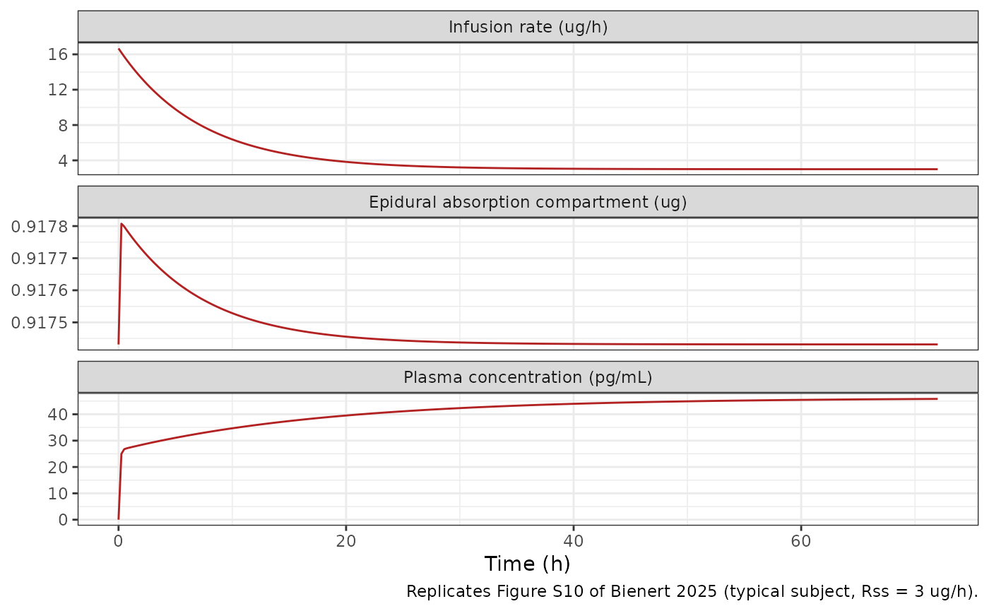
s10_at <- sim_s10 |>
  dplyr::filter(time %in% c(20, 40, 72)) |>
  dplyr::select(time, depot, Cc)
# Figure S10 plasma curve, read off the published panel at 20, 40 and 72 h.
s10_at$Cc_fig <- c(39.5, 44.5, 46)
knitr::kable(s10_at, digits = 3, caption = "Typical-subject Figure S10 values.")| time | depot | Cc | Cc_fig |
|---|---|---|---|
| 20 | 0.917 | 39.531 | 39.5 |
| 40 | 0.917 | 43.973 | 44.5 |
| 72 | 0.917 | 45.831 | 46.0 |
c(
  initial_rate = rss * (1 + ka14 / ka),
  initial_rate_ratio = 1 + ka14 / ka,
  depot_target = rss / ka,
  plasma_ss = 1000 * rss / cl
)
#>       initial_rate initial_rate_ratio       depot_target          plasma_ss
#>         16.6697248          5.5565749          0.9174312         46.2249615

stopifnot(
  # depot is held at Rss / KA by construction. The decaying rate is given as
  # 0.05-h constant-rate steps, which leaves a ripple of a few 1e-4.
  all(abs(sim_s10$depot[sim_s10$time > 0] / (rss / ka) - 1) < 2e-3),
  # Plasma curve matches the published panel.
  all(abs(s10_at$Cc / s10_at$Cc_fig - 1) < 0.10),
  # The paper's 'initial dose rate must be about 5.5 higher'.
  abs((1 + ka14 / ka) - 5.5) < 0.2,
  # Plasma approaches Rss / CL (46.2 pg/mL) by 72 h.
  abs(s10_at$Cc[s10_at$time == 72] / (1000 * rss / cl) - 1) < 0.02
)
The induction dose of 3 / 3.27 = 0.92 ug keeps the
absorption compartment flat, the starting rate is
3 x (1 + 14.9 / 3.27) = 16.7 ug/h (Figure S10 starts just
under 17 ug/h; the Discussion’s “about 5.5 higher”), and plasma rises
from about 27 pg/mL at 1 h towards 1000 x 3 / 64.9 = 46.2
pg/mL, as in Figure S10.
Half-lives of the absorption and disposition processes
The Discussion reports the beta-phase half-life of absorption as 29.7 +/- 5.8 h and of disposition as 13.7 +/- 3.4 h (posterior mean +/- SD of the half-lives computed from each draw of the typical values). The same bi-exponential formula applied to the posterior-mean typical values gives:
q <- exp(mod$theta[["lq"]])
vc <- exp(mod$theta[["lvc"]])
vp <- exp(mod$theta[["lvp"]])
beta_rate <- function(k_out, k_fwd, k_back) {
  s <- k_out + k_fwd + k_back
  0.5 * (s - sqrt(s^2 - 4 * k_back * k_out))
}
thalf_abs <- log(2) / beta_rate(ka, ka14, ka41)
thalf_dis <- log(2) / beta_rate(cl / vc, q / vc, q / vp)
data.frame(
  process = c("absorption (beta)", "disposition (beta)"),
  model_h = c(thalf_abs, thalf_dis),
  paper_mean_h = c(29.7, 13.7),
  paper_sd_h = c(5.8, 3.4)
) |>
knitr::kable(digits = 1)| process | model_h | paper_mean_h | paper_sd_h |
|---|---|---|---|
| absorption (beta) | 27.7 | 29.7 | 5.8 |
| disposition (beta) | 12.7 | 13.7 | 3.4 |
stopifnot(
  abs(thalf_abs - 29.7) < 5.8,
  abs(thalf_dis - 13.7) < 3.4,
  # Flip-flop: absorption is the slower process.
  thalf_abs > thalf_dis
)
The half-lives from the mean typical values sit slightly below the paper’s means, as expected when the paper averages a non-linear function over posterior draws; both are well inside one posterior SD.
Virtual cohort and visual predictive check
The study regimens were individually titrated (the authors’ deposited dataset shows maintenance infusion rates mostly between 0.75 and 3 ug/h, short faster segments of 15-150 ug/h for the initial and supplementary doses, and total infusion durations of 12-74 h), so an exact replication of the Figure 4 VPC is not possible from the published material. As an illustration, 200 virtual patients receive a representative regimen of 10 ug over 10 min followed by 1.5 ug/h for 48 h, sampled on the study’s schedule during and for 72 h after the infusion. The model has no covariates, so no covariate distribution is needed.
obs_during <- c(5 / 60, 0.5, 1, 2, 4, 6, 12, 24, 47.9)
obs_post <- 48 + c(3, 5, 20, 40) / 60
obs_post <- c(obs_post, 48 + c(1, 2, 6, 12, 24, 36, 48, 72))
ev_vpc <- rxode2::et(amt = 10, rate = 60, cmt = "depot") |>
  rxode2::et(time = 1 / 6, amt = 1.5 * (48 - 1 / 6), rate = 1.5, cmt = "depot") |>
  rxode2::et(sort(unique(c(obs_during, obs_post))), cmt = "central")

rxode2::rxSetSeed(20250629)
sim_vpc <- rxode2::rxSolve(mod, ev_vpc, nSub = 200) |>
  as.data.frame()

vpc_sum <- sim_vpc |>
  dplyr::mutate(phase = ifelse(time < 48, "During infusion", "Post infusion"),
                tplot = ifelse(time < 48, time, time - 48)) |>
  dplyr::group_by(phase, tplot) |>
  dplyr::summarise(
    p10 = quantile(sim, 0.1), p50 = quantile(sim, 0.5), p90 = quantile(sim, 0.9),
    .groups = "drop"
  )

ggplot(vpc_sum, aes(tplot)) +
  geom_ribbon(aes(ymin = p10, ymax = p90), fill = "steelblue", alpha = 0.25) +
  geom_line(aes(y = p50), colour = "steelblue", linewidth = 1) +
  facet_wrap(~phase, scales = "free_x") +
  scale_y_log10() +
  labs(
    x = "Time (h)", y = "Sufentanil concentration (pg/mL)",
    caption = paste(
      "Simulated median and 10th-90th percentiles (with residual error);",
      "compare with the layout of Figure 4B of Bienert 2025."
    )
  ) +
  theme_bw()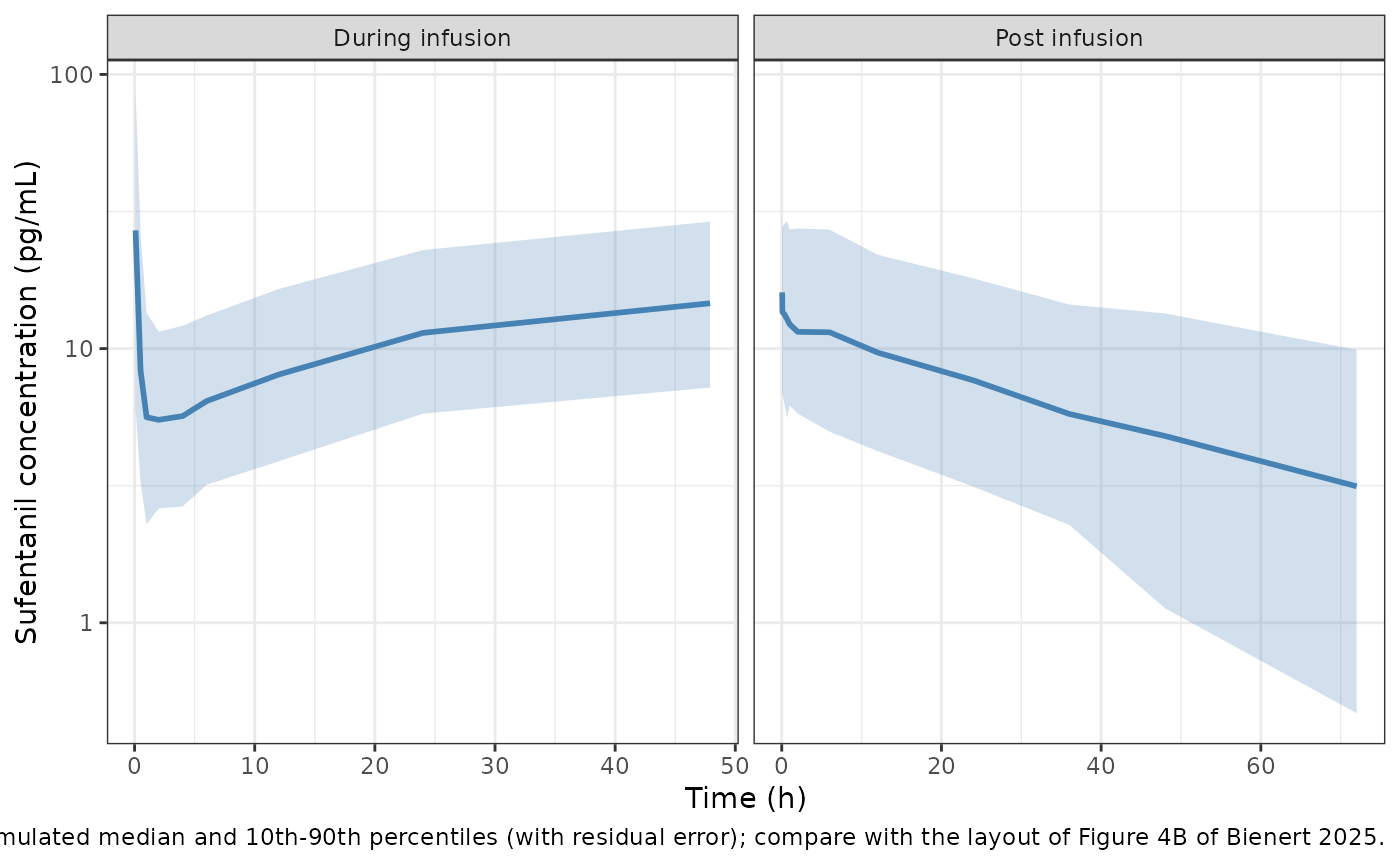
The simulated median rises from a few pg/mL in the first hours to about 10-20 pg/mL at 24-48 h and falls to a few pg/mL 72 h after the infusion stops, the same range as the observed median in Figure 4B.
PKNCA validation
Non-compartmental analysis of the same regimen without residual error (IIV retained), split into the infusion interval (0-48 h) and the post-infusion interval (48-120 h). The paper reports no NCA, so the only published comparator is the terminal half-life: under flip-flop kinetics the late post-infusion decline should approach the absorption beta-phase half-life (29.7 h).
# Cc is the individual prediction (IIV, no residual error); the
# residual-error draw is in the separate `sim` column.
rxode2::rxSetSeed(20250630)
ev_nca <- rxode2::et(amt = 10, rate = 60, cmt = "depot") |>
  rxode2::et(time = 1 / 6, amt = 1.5 * (48 - 1 / 6), rate = 1.5, cmt = "depot") |>
  rxode2::et(sort(unique(c(seq(0, 48, by = 1), 48 + c(0.5, 1, 2, 4, 6, 12, 18, 24, 36, 48, 60, 72)))), cmt = "central")
sim_nca <- rxode2::rxSolve(mod, ev_nca, nSub = 200) |>
  as.data.frame() |>
  dplyr::rename(id = sim.id) |>
  dplyr::mutate(treatment = "10 ug + 1.5 ug/h x 48 h")

conc_df <- sim_nca |>
  dplyr::filter(!is.na(Cc)) |>
  dplyr::select(id, time, Cc, treatment)
dose_df <- data.frame(
  id = rep(unique(conc_df$id), each = 2),
  time = rep(c(0, 1 / 6), times = length(unique(conc_df$id))),
  amt = rep(c(10, 1.5 * (48 - 1 / 6)), times = length(unique(conc_df$id))),
  treatment = "10 ug + 1.5 ug/h x 48 h"
)

conc_obj <- PKNCA::PKNCAconc(conc_df, Cc ~ time | treatment + id, concu = "pg/mL", timeu = "h")
dose_obj <- PKNCA::PKNCAdose(dose_df, amt ~ time | treatment + id, doseu = "ug")
intervals <- data.frame(
  start = c(0, 48),
  end = c(48, 120),
  cmax = c(TRUE, TRUE),
  tmax = c(TRUE, FALSE),
  auclast = c(TRUE, TRUE),
  half.life = c(FALSE, TRUE)
)
nca_res <- PKNCA::pk.nca(PKNCA::PKNCAdata(conc_obj, dose_obj, intervals = intervals))
summary(nca_res)
#>  Interval Start Interval End               treatment   N AUClast (h*pg/mL)
#>               0           48 10 ug + 1.5 ug/h x 48 h 200        528 [51.8]
#>              48          120 10 ug + 1.5 ug/h x 48 h 200        512 [65.3]
#>  Cmax (pg/mL)          Tmax (h) Half-life (h)
#>   15.8 [52.2] 48.0 [1.00, 48.0]             .
#>   15.8 [52.2]                 .   39.6 [28.6]
#>
#> Caption: AUClast, Cmax: geometric mean and geometric coefficient of variation; Tmax: median and range; Half-life: arithmetic mean and standard deviation; N: number of subjects
published <- data.frame(
  treatment = "10 ug + 1.5 ug/h x 48 h",
  half.life = 29.7
)
hl_sim <- as.data.frame(nca_res) |>
  dplyr::filter(PPTESTCD == "half.life", start == 48) |>
  dplyr::select(treatment, PPTESTCD, PPORRES)
cmp <- nlmixr2lib::ncaComparisonTable(
  simulated = hl_sim,
  reference = published,
  by = "treatment",
  params = "half.life",
  units = c(half.life = "h"),
  tolerance_pct = 20
)
knitr::kable(cmp, caption = "Post-infusion terminal half-life: simulated (median) vs the paper's absorption beta-phase half-life. * marks rows differing by >20%.")| NCA parameter | treatment | Reference | Simulated | % diff |
|---|---|---|---|---|
| t½ (h) | 10 ug + 1.5 ug/h x 48 h | 29.7 | 32.2 | +8.4% |
The post-infusion terminal half-life of the simulated cohort is close to the paper’s absorption beta-phase half-life and well above the disposition beta-phase half-life (13.7 h), which is the flip-flop behaviour the model was built to describe.
Assumptions and deviations
-
Posterior means as point estimates. Table 1 reports
the posterior mean and median of each parameter. The model uses the
means, which are the values the paper itself uses for the typical
subject (Discussion: CL 64.9 L/h,
Rss / KAapproximatelyRss / 3.3, KA14 / KA approximately 4.5). -
IIV correlations from the authors’ deposit. The
paper estimates a full 7 x 7 correlation matrix (LKJ(10) prior) but
prints only the SDs. The correlations are the posterior means in the
authors’ public output for the same final model
(
deliv/tables/torsten/3b/parameters-table.csvof github.com/wiczling/sufentanil-epidural). Only the CL-V1 correlation (0.25) has a 90% interval excluding zero; the rest are near zero. The assembled covariance matrix is positive definite. The SDs are the Table 1 values, which match the deposit to two significant figures. - KA41 rounding. Table 1 prints the KA41 mean as 0.14 1/h; the deposit gives 0.135 1/h. The model uses the printed 0.14.
-
Residual error. The paper fits
log(Cobs)with a Student-t error of scale sigma and nu degrees of freedom. This is encoded aslnorm(expSd) + dt(nu); rxode2 uses the same scale parameterisation as Stan.nuis the paper’s name for the degrees of freedom. No canonical name exists for a t-distribution degrees-of-freedom parameter, socheckModelConventions()warns thatnuis not one ofpropSd/addSd/expSd; the warning is expected. -
Epidural distribution compartment. The paper’s A4
exchanges only with the epidural absorption compartment, never with
plasma, a role no registered compartment name covers
(
abs_siteexchanges withcentral;depot2denotes a second dosing route). It is nameddepot_peripheraland declared in the model’spaper_specific_compartments. The paper’s own rate-constant names KA14 and KA41 are kept (ka14,ka41). - Bioavailability. The model assumes complete absorption from the epidural space, as the paper does (Discussion); CL and the volumes are therefore apparent values relative to the epidural dose.
- Illustrative regimen. The VPC and NCA regimen (10 ug over 10 min, then 1.5 ug/h for 48 h) is representative of, not identical to, the individually titrated study regimens, so the VPC is a qualitative comparison with Figure 4B.
- Number of subjects. The paper describes 23 patients; the deposited analysis dataset contains concentration records for 18 of them. The paper does not state that any patient was excluded, and the population metadata reports the 23 described.