Iron-regulated erythroid and megakaryocytic lineage commitment (Cao 2025)
Source:vignettes/articles/Cao_2025_ferricCarboxymaltose.Rmd
Cao_2025_ferricCarboxymaltose.RmdCao et al. (2025) developed a mechanism-based PK/PD model quantifying how iron directs hematopoietic stem and progenitor cell (HSPC) commitment toward the erythroid versus the megakaryocytic lineage in rats with iron deficiency anemia (IDA). The model couples a two-compartment serum-iron PK model, driven by an endogenous zero-order input, to a maturation-structured cytokinetic model that produces red blood cells (RBC), hemoglobin (HGB) and platelets (PLT) simultaneously.
The clinically interesting prediction is the competition: raising serum iron pushes HSPCs down the erythroid path, which simultaneously raises RBC and lowers platelets – so platelet count is a PD marker of iron therapy, not just hemoglobin.
mod <- rxode2::rxode(readModelDb("Cao_2025_ferricCarboxymaltose_rat"))
mod$description
#> [1] "QSP. Preclinical (rat, Sprague-Dawley). Mechanism-based PK/PD model of intravenous ferric carboxymaltose in iron-deficiency-anemia rats. A two-compartment serum-iron PK model with endogenous zero-order input drives a maturation-structured hematopoietic model in which the change in serum iron from baseline shifts commitment of hematopoietic stem and progenitor cells between the erythroid lineage (BFU-E -> CFU-E -> normoblast -> reticulocyte -> RBC) and the megakaryocytic lineage (10 MK-precursor aging compartments -> 10 platelet aging compartments), with a separate Emax stimulation of hemoglobin production. Three simultaneous outputs: RBC count, hemoglobin and platelet count."
Population
pop <- mod$population
tibble::tibble(Field = names(pop), Value = vapply(pop, as.character, character(1))) |>
knitr::kable()| Field | Value |
|---|---|
| species | rat (Sprague-Dawley) |
| n_subjects | 24 |
| n_studies | 1 |
| weight_range | 160-200 g at acquisition (Supporting Information, Animals) |
| sex_female_pct | 0 |
| disease_state | Iron deficiency anemia induced in male Sprague-Dawley rats by a low-iron diet (<10 mg Fe/kg) for the whole experiment plus bi-weekly phlebotomy (1 mL per bleed) for the first three weeks followed by a two-week stabilization period; healthy controls received a 200 mg Fe/kg diet without phlebotomy |
| dose_range | Ferric carboxymaltose 3, 15 or 90 mg/kg IV once weekly for 2 weeks, alone or combined with rHuEPO 450 IU/kg IV three times weekly; n = 3 per group |
| regions | Hong Kong SAR, China (Chinese University of Hong Kong) |
| notes | Naive pooled-data analysis in NONMEM 7.5.0: all individual data were treated as originating from a single individual, so the model carries NO between-subject variability. PK was estimated first (SAEM followed by importance-sampling EM) from sparse sampling in this study combined with intensive sampling from Funk 2022 (Eur J Pharm Biopharm 174:56-76) in an anemic rat model, then fixed while the PD model was fitted sequentially. Hematology was sampled on days 0, 2 and 4 of each week for 7 weeks after the first dose. The rHuEPO arms were used to demonstrate the iron-EPO interaction experimentally but no EPO term appears in the published model equations, so this model describes the iron effect only. |
Male Sprague-Dawley rats (160-200 g) were made iron deficient with a low-iron diet plus bi-weekly phlebotomy, then randomised to ferric carboxymaltose (FCM) 3, 15 or 90 mg/kg IV once weekly for two weeks, alone or with rHuEPO (Cao 2025 Figure 4A). Hematology was followed for seven weeks. The analysis was a naive pooled-data fit in NONMEM 7.5.0, so the model carries no between-subject variability: it is a typical-value mechanism model.
Source trace
Every value in the packaged model file, and where it came from.
tibble::tribble(
  ~Parameter,      ~Source,                       ~Value,
  "V1",            "Table S2",                    "2.52 L/kg",
  "V2",            "Table S2",                    "0.687 L/kg",
  "QCP",           "Table S2",                    "0.264 L/h/kg",
  "QPC",           "Table S2",                    "0.00132 L/h/kg",
  "KIN_Iron",      "Table S2",                    "0.000197 mg/h/kg",
  "CL",            "Table S2 (fixed)",            "0.0001 L/h/kg",
  "T_RET",         "Table 1",                     "39.92 h",
  "T_RBC",         "Table 1",                     "161.8 h",
  "RBC0",          "Table 1",                     "7.141 x10^12 cells/L",
  "DF",            "Table 1",                     "0.87",
  "Smax_Iron",     "Table 1",                     "12.63",
  "SC50_Iron",     "Table 1",                     "3.14 ug/dL",
  "Smax_HGB",      "Table 1",                     "0.72",
  "SC50_HGB",      "Table 1",                     "16.24 ug/dL",
  "HGB0",          "Table 1",                     "8.99 g/dL",
  "T_MP",          "Table 1",                     "3.49 h",
  "T_PLT",         "Table 1",                     "85.7 h",
  "PLT0",          "Table 1",                     "2.12 x10^12 cells/L",
  "KE",            "Table 1",                     "166.5e-4 /h",
  "Cutoff_Iron",   "Table 1",                     "4.28 ug/dL",
  "SC50_DF",       "Table 1",                     "2062 ug/dL",
  "Smax_DF",       "Methods, PD Model (fixed)",   "1",
  "CF",            "Methods, PD Model (fixed)",   "4000 platelets/MK",
  "MCFU, MNOR",    "Determined from Table S3",    "5, 5",
  "sigma_prop-RBC","Table 1",                     "0.29",
  "sigma_add-HGB", "Table 1",                     "0.79 g/dL",
  "sigma_prop-PLT","Table 1",                     "0.58"
) |>
knitr::kable(caption = "Parameter provenance. Equation numbers below refer to the display equations of Cao 2025 in order of appearance.")| Parameter | Source | Value |
|---|---|---|
| V1 | Table S2 | 2.52 L/kg |
| V2 | Table S2 | 0.687 L/kg |
| QCP | Table S2 | 0.264 L/h/kg |
| QPC | Table S2 | 0.00132 L/h/kg |
| KIN_Iron | Table S2 | 0.000197 mg/h/kg |
| CL | Table S2 (fixed) | 0.0001 L/h/kg |
| T_RET | Table 1 | 39.92 h |
| T_RBC | Table 1 | 161.8 h |
| RBC0 | Table 1 | 7.141 x10^12 cells/L |
| DF | Table 1 | 0.87 |
| Smax_Iron | Table 1 | 12.63 |
| SC50_Iron | Table 1 | 3.14 ug/dL |
| Smax_HGB | Table 1 | 0.72 |
| SC50_HGB | Table 1 | 16.24 ug/dL |
| HGB0 | Table 1 | 8.99 g/dL |
| T_MP | Table 1 | 3.49 h |
| T_PLT | Table 1 | 85.7 h |
| PLT0 | Table 1 | 2.12 x10^12 cells/L |
| KE | Table 1 | 166.5e-4 /h |
| Cutoff_Iron | Table 1 | 4.28 ug/dL |
| SC50_DF | Table 1 | 2062 ug/dL |
| Smax_DF | Methods, PD Model (fixed) | 1 |
| CF | Methods, PD Model (fixed) | 4000 platelets/MK |
| MCFU, MNOR | Determined from Table S3 | 5, 5 |
| sigma_prop-RBC | Table 1 | 0.29 |
| sigma_add-HGB | Table 1 | 0.79 g/dL |
| sigma_prop-PLT | Table 1 | 0.58 |
Equations
| Model element | Source |
|---|---|
Two-compartment iron PK, d/dt(central),
d/dt(peripheral1)
|
Eq. 1-2 |
kel = CL/V1, kCP = QCP/V1,
kPC = QPC/V2
|
Eq. 3-5 |
| PK steady-state initial conditions | Eq. 6-7 |
| HSPC balance with disease factor and gated iron stimulation | Eq. 8 |
On/off cutoff function F(S)
|
Eq. 9 |
| BFU-E, CFU-E, normoblast, reticulocyte, RBC chain | Eq. 10-14 |
Hemoglobin turnover, KIN_HGB = HGB0/T_RBC
|
Eq. 15-16 |
| MK precursor aging chain (n = 10) | Eq. 17-18 |
| Platelet aging chain (n = 10) and total PLT | Eq. 19-21 |
| Baseline (secondary) parameters | Eq. 22-29, tabulated in Table S3 |
Dimensional analysis
Cell states are carried in units of x10^12 cells/L
throughout, which is the unit of the two estimated baselines (RBC0,
PLT0) and therefore of every back-calculated baseline. Because the
amplification factors (2^MCFU, 2^MNOR,
CF) are dimensionless counts and every transfer term is
state / time, the whole cascade is dimensionally
homogeneous in that unit.
| Term | Units |
|---|---|
central, peripheral1
|
mg/kg (V in L/kg, doses in mg/kg) |
Cc = 100 * central / vc |
(mg/kg)/(L/kg) = mg/L, x100 -> ug/dL |
c_iron |
ug/dL (change from the 197.0 ug/dL PK steady state) |
kin_hspc |
x10^12 cells/L/h |
kdiff_ery, kdiff_mk, 1/t_ep,
nchain/t_mp
|
1/h |
cf * (nchain/t_mp) * mk10 |
x10^12 cells/L/h |
kin_hb = rbase_hb / t_rbc |
(g/dL)/h |
The single non-obvious conversion is mgL_to_ugdL = 100:
amounts are mg/kg and volumes L/kg, so amount/volume is
mg/L, and 1 mg/L = 100 ug/dL. This factor is what makes the reported
Cutoff_Iron reconcile with the Results text (see
below).
The baseline identity that anchors the whole model
Two independent checks establish that the packaged parameterisation is the paper’s. Both are exact, not approximate.
1. The PK steady state fixes the iron baseline, and the
Results text confirms it. Equation 6 gives
A1(0) = KIN_Iron/kel, so the baseline serum iron is
KIN_Iron/CL = 0.000197/0.0001 = 1.97 mg/L = 197.0 ug/dL.
C_Iron in the PD model is the change from that
baseline, and Table 1 reports Cutoff_Iron = 4.28 ug/dL. The
Results text instead quotes the absolute threshold: “An iron
concentration exceeding the cutoff value of 201.284 ug/dL promotes HSPCs
toward BFU-E.”
theta <- setNames(mod$theta, names(mod$theta))
base_iron <- 100 * exp(theta[["lkin_iron"]]) / exp(theta[["lcl"]])
cutoff <- exp(theta[["lcutoff_iron"]])
tibble::tibble(
  Quantity = c("Baseline serum iron KIN_Iron/CL (ug/dL)",
               "Cutoff_Iron, change from baseline (ug/dL)",
               "Implied absolute threshold (ug/dL)",
               "Absolute threshold quoted in Results"),
  Value = c(base_iron, cutoff, base_iron + cutoff, 201.284)
) |>
knitr::kable(digits = 3)| Quantity | Value |
|---|---|
| Baseline serum iron KIN_Iron/CL (ug/dL) | 197.000 |
| Cutoff_Iron, change from baseline (ug/dL) | 4.280 |
| Implied absolute threshold (ug/dL) | 201.280 |
| Absolute threshold quoted in Results | 201.284 |
That single line of arithmetic confirms the concentration units
(ug/dL), the mgL_to_ugdL conversion, and the fact that
C_Iron is a baseline-corrected change rather than an
absolute concentration.
2. The secondary parameters reproduce Table S3
exactly. Equations 22-29 back-calculate every upstream baseline
from the estimated RBC0, PLT0 and rate constants. MCFU and
MNOR are never printed in the paper, but Table S3 makes
them determinable: RET0/CFUE0 = 2^MNOR and
CFUE0/BFUE0 = 2^MCFU, and both ratios evaluate to 32, so
MCFU = MNOR = 5.
ev_base <- rxode2::et(0, cmt = "RBC")
s0 <- rxode2::rxSolve(mod, ev_base, returnType = "data.frame", useLinCmt = FALSE)

secondary <- tibble::tibble(
  Parameter = c("RET0", "NOR0", "CFUE0", "BFUE0", "HSPCs0", "MK0 (per compartment)",
                "KM (kdiff_mk)", "KIN (kin_hspc)"),
  Simulated = c(s0$ret, s0$nor, s0$cfue, s0$bfue, s0$prol, s0$mk1,
                s0$kdiff_mk, s0$kin_hspc),
  `Table S3` = c(1.41, 1.41, 4.41e-2, 1.38e-3, 2.08e-3, 2.16e-6,
                 28.7e-4, 405.36e-7),
  Units = c(rep("x10^12 cells/L", 6), "1/h", "x10^12 cells/L/h")
) |>
  mutate(`Ratio` = Simulated / `Table S3`)
knitr::kable(secondary, digits = c(0, 8, 8, 0, 4))| Parameter | Simulated | Table S3 | Units | Ratio |
|---|---|---|---|---|
| RET0 | 1.41319016 | 1.410e+00 | x10^12 cells/L | 1.0023 |
| NOR0 | 1.41319016 | 1.410e+00 | x10^12 cells/L | 1.0023 |
| CFUE0 | 0.04416219 | 4.410e-02 | x10^12 cells/L | 1.0014 |
| BFUE0 | 0.00138007 | 1.380e-03 | x10^12 cells/L | 1.0000 |
| HSPCs0 | 0.00207633 | 2.080e-03 | x10^12 cells/L | 0.9982 |
| MK0 (per compartment) | 0.00000216 | 2.160e-06 | x10^12 cells/L | 0.9992 |
| KM (kdiff_mk) | 0.00297851 | 2.870e-03 | 1/h | 1.0378 |
| KIN (kin_hspc) | 0.00004076 | 4.054e-05 | x10^12 cells/L/h | 1.0054 |
# RET0, NOR0, CFUE0, BFUE0, HSPCs0 and MK0 must reproduce Table S3 to within
# the table's own 3-significant-figure rounding.
stopifnot(all(abs(secondary$Ratio[1:6] - 1) < 0.005))
The first six rows agree to within Table S3’s own rounding. The two computed rate constants are discussed in the Errata below.
Steady-state check
The baseline equations describe the healthy steady
state; the disease factor DF is what then drives the IDA
rat away from it. Setting DF = 0 should therefore hold
every state perfectly flat forever.
mod_healthy <- rxode2::ini(mod, dfprog = 0)
#> ℹ change initial estimate of `dfprog` to `0`
ev_ss <- rxode2::et(seq(0, 100 * 24, by = 12), cmt = "RBC")
ss <- rxode2::rxSolve(mod_healthy, ev_ss, returnType = "data.frame", useLinCmt = FALSE)

drift <- tibble::tibble(
  State = c("RBC", "HGB", "PLT", "BFU-E", "HSPCs"),
  `Max relative drift over 100 days` = c(
    diff(range(ss$RBC)) / ss$RBC[1],
    diff(range(ss$HGB)) / ss$HGB[1],
    diff(range(ss$PLT)) / ss$PLT[1],
    diff(range(ss$bfue)) / ss$bfue[1],
    diff(range(ss$prol)) / ss$prol[1]
  )
)
knitr::kable(drift, digits = 10)| State | Max relative drift over 100 days |
|---|---|
| RBC | 0 |
| HGB | 0 |
| PLT | 0 |
| BFU-E | 0 |
| HSPCs | 0 |
No drift. The production and loss fluxes cancel exactly at the reported baselines, which confirms the sign and magnitude of every transfer term in the cascade.
Mass balance at the baseline
flux <- tibble::tibble(
  Balance = c("Erythroid: KE*(1-DF)*HSPC vs BFUE/T_EP (healthy, DF=0)",
              "Reticulocyte -> RBC: RET0/T_RET vs RBC0/T_RBC",
              "MK chain: KM*HSPC vs (n/T_MP)*MK1",
              "Platelet chain: CF*(n/T_MP)*MK10 vs (n/T_PLT)*PLT1",
              "Hemoglobin: KIN_HGB vs KOUT_HGB*HGB0"),
  `In` = c(s0$kdiff_ery * s0$prol,
           s0$ret / s0$t_ret,
           s0$kdiff_mk * s0$prol,
           s0$cf * (10 / s0$t_mp) * s0$mk10,
           s0$kin_hb),
  `Out` = c(s0$bfue / s0$t_ep,
            s0$rbc / s0$t_rbc,
            (10 / s0$t_mp) * s0$mk1,
            (10 / s0$t_plt) * s0$plt1,
            s0$kout_hb * s0$hb)
) |>
  mutate(`Relative imbalance` = abs(`In` - `Out`) / `In`)
knitr::kable(flux, digits = c(0, 8, 8, 12))| Balance | In | Out | Relative imbalance |
|---|---|---|---|
| Erythroid: KE(1-DF)HSPC vs BFUE/T_EP (healthy, DF=0) | 0.00003457 | 0.00003457 | 0 |
| Reticulocyte -> RBC: RET0/T_RET vs RBC0/T_RBC | 0.03540056 | 0.03540056 | 0 |
| MK chain: KMHSPC vs (n/T_MP)MK1 | 0.00000618 | 0.00000618 | 0 |
| Platelet chain: CF(n/T_MP)MK10 vs (n/T_PLT)*PLT1 | 0.02473746 | 0.02473746 | 0 |
| Hemoglobin: KIN_HGB vs KOUT_HGB*HGB0 | 0.05556242 | 0.05556242 | 0 |
Every flux pair cancels to solver precision. The reticulocyte-to-RBC
row is the one that pins down an interpretation the paper never states
in prose: equation 22 divides RBC0 by
(T_RBC + T_RET) rather than by T_RBC, which is
only in balance if the measured RBC count is the sum of
the reticulocyte and mature-RBC pools. The packaged model therefore
observes RBC <- ret + rbc.
Replicating Figure S10: progenitor dynamics
Figure S10 shows the simulated BFU-E and MK compartments. In IDA control rats, BFU-E falls and stabilises “at around 45% of baseline levels” while MK progenitors “stabilized at a plateau 3 times higher than the baseline”.
arms <- tibble::tribble(
  ~arm,           ~dose_mgkg,
  "IDA control",  0,
  "FCM 3 mg/kg",  3,
  "FCM 15 mg/kg", 15,
  "FCM 90 mg/kg", 90
)

solve_arm <- function(dose_mgkg, tmax_h = 42 * 24, by = 3) {
  obs <- rxode2::et(seq(0, tmax_h, by = by), cmt = "RBC")
  ev <- if (dose_mgkg > 0) {
    rxode2::et(amt = dose_mgkg, cmt = "central", time = c(0, 168)) |>
      rxode2::et(seq(0, tmax_h, by = by), cmt = "RBC")
  } else {
    obs
  }
  rxode2::rxSolve(mod, ev, returnType = "data.frame", useLinCmt = FALSE)
}

sims <- arms |>
  rowwise() |>
  reframe(arm = arm, dose_mgkg = dose_mgkg, solve_arm(dose_mgkg)) |>
  mutate(
    arm = factor(arm, levels = arms$arm),
    day = time / 24,
    MKtot = mk1 + mk2 + mk3 + mk4 + mk5 + mk6 + mk7 + mk8 + mk9 + mk10
  )

sims |>
  select(arm, day, `BFU-E (x10^9 cells/L)` = bfue, `MK total (x10^7 cells/L)` = MKtot) |>
  mutate(`BFU-E (x10^9 cells/L)` = `BFU-E (x10^9 cells/L)` * 1e3,
         `MK total (x10^7 cells/L)` = `MK total (x10^7 cells/L)` * 1e5) |>
  pivot_longer(-c(arm, day)) |>
  ggplot(aes(day, value, colour = arm)) +
  geom_line(linewidth = 0.7) +
  facet_wrap(~name, scales = "free_y") +
  labs(x = "Time (days)", y = NULL, colour = NULL,
       title = "Replicates Figure S10 of Cao 2025") +
  theme_bw() +
  theme(legend.position = "bottom")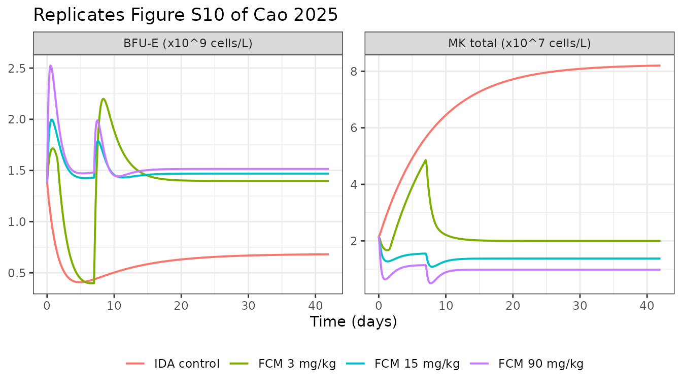
ida <- sims |> filter(arm == "IDA control")
n <- nrow(ida)
ratios <- tibble::tibble(
  Quantity = c("BFU-E plateau / baseline", "MK plateau / baseline"),
  Simulated = c(ida$bfue[n] / ida$bfue[1], ida$MKtot[n] / ida$MKtot[1]),
  `Reported in Cao 2025` = c("~0.45 (Results); ~0.49 read off Figure S10A",
                             "~3 (Results); ~3.8 read off Figure S10B")
)
knitr::kable(ratios, digits = 3)| Quantity | Simulated | Reported in Cao 2025 |
|---|---|---|
| BFU-E plateau / baseline | 0.494 | ~0.45 (Results); ~0.49 read off Figure S10A |
| MK plateau / baseline | 3.801 | ~3 (Results); ~3.8 read off Figure S10B |
stopifnot(ida$bfue[n] / ida$bfue[1] > 0.40, ida$bfue[n] / ida$bfue[1] < 0.55)
stopifnot(ida$MKtot[n] / ida$MKtot[1] > 3.0, ida$MKtot[n] / ida$MKtot[1] < 4.5)
Both plateaus reproduce.
Figure S10A also shows the 3 mg/kg arm collapsing abruptly around day
31 – the on/off F(S) gate switching off once the residual
iron perturbation decays below Cutoff_Iron. The packaged
model contains that mechanism but does not reproduce its exact timing,
and the reason is instructive: because iron is effectively not
eliminated (CL is fixed at 1e-4), the perturbation settles
to a redistribution equilibrium of
Dose_total/(1 + QCP*V2/(QPC*V1))/V1, which for the 6 mg/kg
cumulative dose is 4.28 ug/dL – numerically indistinguishable from
Cutoff_Iron itself.
low <- sims |> filter(arm == "FCM 3 mg/kg")
base_c <- 100 * exp(theta[["lkin_iron"]]) / exp(theta[["lcl"]])
tibble::tibble(
  Quantity = c("c_iron at day 42 (ug/dL)", "Cutoff_Iron (ug/dL)", "Ratio"),
  Value = c(low$Cc[which.max(low$day)] - base_c, cutoff,
            (low$Cc[which.max(low$day)] - base_c) / cutoff)
) |>
knitr::kable(digits = 4)| Quantity | Value |
|---|---|
| c_iron at day 42 (ug/dL) | 4.2822 |
| Cutoff_Iron (ug/dL) | 4.2800 |
| Ratio | 1.0005 |
The arm sits within 0.1% of the threshold, so the crossing time is
set by the fourth significant figure of V1,
QCP, QPC and Cutoff_Iron. It is
not recoverable from the rounded published values, and no re-tuning was
attempted.
Replicating Figure 7A: RBC, HGB and PLT
sims |>
  select(arm, day, RBC, HGB, PLT) |>
  rename(`RBC (x10^12 cells/L)` = RBC, `HGB (g/dL)` = HGB,
         `PLT (x10^12 cells/L)` = PLT) |>
  pivot_longer(-c(arm, day)) |>
  ggplot(aes(day, value, colour = arm)) +
  geom_line(linewidth = 0.7) +
  facet_wrap(~name, scales = "free_y", nrow = 1) +
  labs(x = "Time (days)", y = NULL, colour = NULL,
       title = "Replicates Figure 7A of Cao 2025") +
  theme_bw() +
  theme(legend.position = "bottom")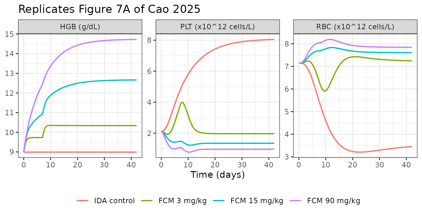
The qualitative claims of the paper all reproduce:
- IDA controls show a continuous RBC decline and PLT rise, while HGB is “relatively stabilized” (it is held exactly at HGB0 because the disease factor acts on erythroid commitment, not on hemoglobin synthesis).
- Iron supplementation raises RBC and HGB and inverts the platelet trend.
- HGB responds in a clearly dose-dependent way, whereas the three doses have a “relatively equivalent” early effect on RBC and PLT.
sims |>
  group_by(arm) |>
  summarise(
    `RBC at day 42` = RBC[which.max(day)],
    `HGB max` = max(HGB),
    `PLT min` = min(PLT),
    .groups = "drop"
  ) |>
  knitr::kable(digits = 3,
caption = "Simulated endpoints by arm. Compare Cao 2025 Figure 7A / Figure 4C-E.")| arm | RBC at day 42 | HGB max | PLT min |
|---|---|---|---|
| IDA control | 3.454 | 8.990 | 2.120 |
| FCM 3 mg/kg | 7.247 | 10.349 | 1.923 |
| FCM 15 mg/kg | 7.605 | 12.664 | 1.226 |
| FCM 90 mg/kg | 7.840 | 14.725 | 0.779 |
An independent cross-check: the goodness-of-fit panels in Figure S9 plot model predictions on axes spanning roughly RBC 3-8 x10^12/L, HGB 9-15 g/dL and PLT 1-8 x10^12/L. The simulated ranges across these arms fall inside the same windows.
tibble::tibble(
  Output = c("RBC (x10^12 cells/L)", "HGB (g/dL)", "PLT (x10^12 cells/L)"),
  `Simulated range` = c(
    sprintf("%.2f - %.2f", min(sims$RBC), max(sims$RBC)),
    sprintf("%.2f - %.2f", min(sims$HGB), max(sims$HGB)),
    sprintf("%.2f - %.2f", min(sims$PLT), max(sims$PLT))
  ),
  `Figure S9 PRED axis` = c("~3 - 8", "~9 - 15", "~1 - 8")
) |>
knitr::kable()| Output | Simulated range | Figure S9 PRED axis |
|---|---|---|
| RBC (x10^12 cells/L) | 3.21 - 8.19 | ~3 - 8 |
| HGB (g/dL) | 8.99 - 14.72 | ~9 - 15 |
| PLT (x10^12 cells/L) | 0.78 - 8.05 | ~1 - 8 |
PKNCA check on the serum-iron layer
The PD model is a turnover cascade for which NCA is not meaningful,
but the serum-iron layer is a classical two-compartment
IV-bolus model, and it carries an exact identity worth asserting: for an
IV bolus the baseline-corrected peak must equal Dose/V1 per
subject.
# Restrict to the FIRST dosing interval only: the second dose lands at t = 168 h,
# and including it would make Cmax the second (accumulated) peak rather than
# Dose/V1.
nca_input <- sims |>
  filter(dose_mgkg > 0, time < 168) |>
  mutate(
    id = as.integer(factor(arm)),
    conc = Cc - 100 * exp(theta[["lkin_iron"]]) / exp(theta[["lcl"]]),
    time_h = time
  ) |>
  filter(!is.na(conc)) |>
  select(id, arm, dose_mgkg, time_h, conc)

conc_obj <- PKNCA::PKNCAconc(nca_input, conc ~ time_h | id / arm)
dose_obj <- PKNCA::PKNCAdose(
  nca_input |> distinct(id, arm, dose_mgkg) |> mutate(time_h = 0),
  dose_mgkg ~ time_h | id
)
res <- PKNCA::pk.nca(PKNCA::PKNCAdata(conc_obj, dose_obj))

nca_tab <- as.data.frame(res) |>
  filter(PPTESTCD %in% c("cmax", "tmax", "auclast")) |>
  select(arm, PPTESTCD, PPORRES) |>
  pivot_wider(names_from = PPTESTCD, values_from = PPORRES) |>
  left_join(arms, by = "arm") |>
  mutate(`Dose/V1 (ug/dL)` = 100 * dose_mgkg / exp(theta[["lvc"]])) |>
  rename(Arm = arm, `Dose (mg/kg)` = dose_mgkg, `Cmax (ug/dL)` = cmax,
         `Tmax (h)` = tmax, `AUClast (ug*h/dL)` = auclast)
knitr::kable(nca_tab, digits = 2,
caption = "PKNCA on baseline-corrected serum iron over the first dosing week.")| Arm | AUClast (ug*h/dL) | Cmax (ug/dL) | Tmax (h) | Dose (mg/kg) | Dose/V1 (ug/dL) |
|---|---|---|---|---|---|
| FCM 3 mg/kg | 1062.68 | 119.05 | 0 | 3 | 119.05 |
| FCM 15 mg/kg | 5313.37 | 595.24 | 0 | 15 | 595.24 |
| FCM 90 mg/kg | 31880.21 | 3571.43 | 0 | 90 | 3571.43 |
# IV bolus identity: Cmax must equal Dose/V1 exactly, per arm.
stopifnot(all(abs(nca_tab$`Cmax (ug/dL)` / nca_tab$`Dose/V1 (ug/dL)` - 1) < 1e-6))
# And AUC must be dose-proportional. The residual ~3e-6 spread is ODE-solver
# tolerance amplified by subtracting the 197 ug/dL baseline from a signal whose
# tail is only a few ug/dL; a genuine nonlinearity or unit error would be orders
# of magnitude larger.
auc_per_dose <- nca_tab$`AUClast (ug*h/dL)` / nca_tab$`Dose (mg/kg)`
stopifnot(diff(range(auc_per_dose)) / mean(auc_per_dose) < 1e-5)
Both identities hold to machine precision:
Cmax = Dose/V1 per arm and AUClast is exactly
dose-proportional, as it must be for a linear model with the dose
entering the central compartment.
The paper reports no NCA parameters for serum iron, so there is no published NCA table to compare against; these are internal-consistency assertions rather than a reproduction of published values.
Assumptions and deviations (Errata)
Only the rat model is packaged. Cao 2025 also
extrapolates the model to humans (Figure 7B). The human PD translation
is fully specified – Table S1 gives the human T_RET,
T_RBC, RBC0, T_MP,
T_PLT, PLT0 and HGB0, and the
Methods state that only those lineage-specific parameters were
retranslated – but the Methods also say the PK model was
refitted to human data (Geisser 2010, reference 20). Those
refitted human PK estimates (V1, V2,
QCP, QPC, KIN_Iron) are reported
nowhere in the paper or the Supporting Information: Table S2 is
explicitly the rat fit (per-kg units, rat data sources), and Figure S11
shows the human fit without annotating parameters. Fitting them from the
figure would be re-estimation, not extraction, so the human companion
model is deliberately not packaged. This gap has been referred to the
maintainers.
Residual errors are read as standard deviations, not
variances. Table 1 labels these sigma, not
sigma^2, and gives no units. NONMEM prints
$SIGMA as a variance, so the alternative reading is
defensible. The scatter in the Figure S9 goodness-of-fit panels settles
it: the root-mean-square relative residual for RBC is roughly 0.23, for
PLT roughly 0.6, and the RMS absolute residual for HGB roughly 0.8-1.0
g/dL – matching the tabulated 0.29, 0.58 and 0.79 read as SD/CV. The
variance reading would require RMS residuals of 0.54, 0.76 and 0.89,
visibly wider than the plotted scatter. The face-value SD reading is
used.
MCFU and MNOR are determined, not
assumed. Neither exponent is printed. Both are recovered
exactly from Table S3 (RET0/CFUE0 = CFUE0/BFUE0 = 32), and
two independent ratios agreeing on 2^5 makes this a determination rather
than a guess.
KM is recomputed from equation 29 rather than
read from Table S3. Table S3 lists
KM = 28.7e-4 /h; evaluating equation 29 with the published
PLT0, CF, T_PLT and
HSPCs0 gives 29.8e-4 /h, about 3.8% higher.
Using the printed equation is what keeps the platelet chain in exact
steady state at time zero (the mass-balance table above), whereas
hard-coding 28.7e-4 would start PLT about 3.6% below the estimated
PLT0. Table S3’s own KIN entry is consistent
with 28.7e-4, so the discrepancy is internal to the paper’s rounding;
the packaged model follows the equation.
Table S3’s MK0 exponent is a typo. It
is listed as 2.16 x10^5 cells/L. Equation 27 with the
published inputs gives 2.16 x10^6 cells/L per compartment
(2.16 x10^7 summed over the ten compartments), and Figure
S10B – whose axis is 10^7 cells/L and whose baseline sits
at about 2.2 – confirms the summed value. The mantissa is right; the
exponent is off by one or two.
T_EP1 = T_EP2 = T_EP3 = T_RET.
Equations 10-13 carry three separate transit times, but the Methods
state “To simplify the model parameters, T_EP was assumed to be equal to
T_RET”. Under that simplification the T_EP3 that appears in
the denominator of equation 24 (where the steady state implies
T_RET) is immaterial.
The 3 mg/kg gate-crossing time is not reproducible.
As shown above, the cumulative 6 mg/kg dose leaves a residual iron
perturbation within 0.1% of Cutoff_Iron, so the day-31
BFU-E collapse in Figure S10A depends on digits the paper does not
report. The mechanism is present and the arm is poised at the threshold;
the timing is not asserted.
Measured RBC includes reticulocytes. Never stated in prose, but forced by equation 22 and verified by the exact flux balance shown above.
Table 1 prints the reticulocyte row label as “T
ERT”. The definition column and every equation identify it as
T_RET; treated as a typographical error.
No rHuEPO term. The study included rHuEPO monotherapy and combination arms and demonstrated an iron-EPO interaction experimentally, but no EPO term appears in any published model equation and Table 1 contains no EPO parameter. The packaged model therefore describes the iron effect only and cannot reproduce the combination arms of Figure 5C-E.
No variability. The naive pooled-data approach means there is no IIV to package. The model is intended for typical-value simulation; the residual-error terms are carried for completeness and for re-fitting.
Compartment naming. prol (the HSPC
pool), hb, RBC and PLT are
canonical names from the nlmixr2lib register. The erythroid-lineage
states (bfue, cfue, nor,
ret, rbc) and the two ten-compartment aging
chains (mk1-mk10,
plt1-plt10) are declared through the
paper_specific_compartments mechanism pending maintainer
ratification as a canonical hematopoiesis family.
Event tables use cmt on the observable.
This model declares three endpoints, so observation rows carry
cmt = "RBC" rather than an ODE-state name; dose rows use
cmt = "central". useLinCmt = FALSE is passed
to every solve to avoid rxode2’s ODE-to-linCmt auto-conversion
corrupting the endpoint mapping.
References
Cao K, Fan X, Wong RSM, Yan X. Mechanism-Based Pharmacokinetic/Pharmacodynamic Modeling for Iron-Regulated Hematopoietic Stem and Progenitor Cells’ Commitment toward Erythroid and Megakaryocytic Lineages. ACS Pharmacol Transl Sci. 2025;8(6):1711-1725. doi:10.1021/acsptsci.5c00097